What Is Geospatial Analysis? A Complete Guide to Methods, Tools, and Applications (Update 2026)

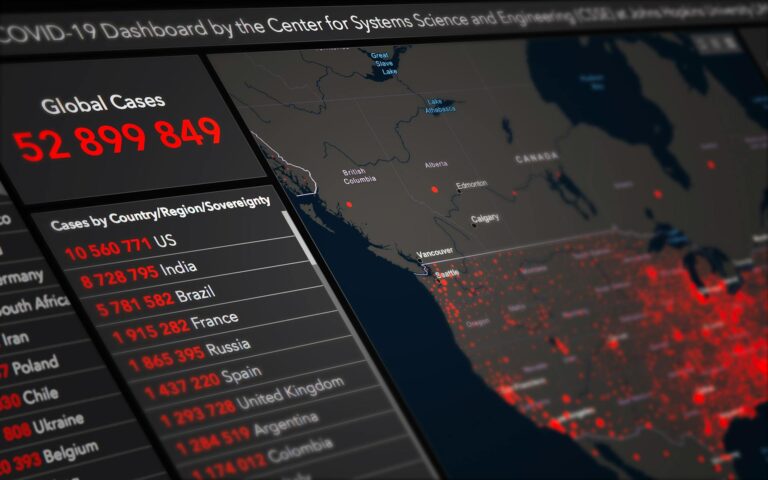
Two hospitals serve the same city. Both report identical patient volumes. One is overwhelmed. The other has spare capacity.

The difference isn’t in the numbers. It’s in where the patients live relative to each hospital — distances, road access, population distribution. None of that shows up in a spreadsheet until you map it.

That’s the problem geospatial analysis exists to solve.

What Is Geospatial Analysis?

Geospatial analysis is the process of examining, manipulating, and interpreting spatial data to extract patterns, relationships, and insights that have a geographic component. It is the analytical layer of the geospatial field — the bridge between raw location data and actionable knowledge.

Think of the distinction this way. A map shows you where things are.

Geospatial analysis answers the harder questions:

• why are they there,
• how do they relate to other things in space,
• what patterns emerge across the landscape, and
• what is likely to happen next?

A map of hospital locations is useful. A geospatial analysis that calculates which neighborhoods fall outside a 30-minute drive of emergency care, weighted by road network, traffic conditions, and population density, is actionable.

The field draws on methods from geography, mathematics, statistics, and computer science.

It operates on both vector data (points, lines, polygons representing discrete features) and raster data (continuous grids representing surfaces like elevation, temperature, or vegetation density). And it scales from a simple buffer query run on a laptop to a continental-scale change detection analysis running on cloud infrastructure.

What makes geospatial analysis distinct from every other form of data analysis is its treatment of location as a first-class analytical variable, not just a label or a filter, but a dimension that carries its own logic, relationships, and patterns.

How Is Geospatial Analysis Different From Regular Data Analysis?

Regular data analysis works with rows and columns: attributes, values, and relationships between variables. It asks questions like: how many, how much, what proportion, which group performs better? These are powerful questions, and standard analytical tools answer them well.

Geospatial analysis adds a dimension that those tools don’t natively handle: location. And location changes everything, because the world is not uniform.

Two data points that look identical in a spreadsheet can behave completely differently when their spatial relationship is considered.

A property inside a flood zone and one outside it have identical attributes until you map them, because then their risk profiles diverge entirely.

A health outcome in a neighborhood with no nearby green space and the same outcome in a well-served neighborhood tell completely different stories about environmental exposure.

A retail store within 500 meters of a transit stop and one two kilometers away face fundamentally different foot traffic dynamics.

This is what geographers call spatial dependence. It is the principle that things that are near each other tend to be more similar than things that are far apart, and that location itself carries predictive power. Standard data analysis ignores this. Geospatial analysis is built around it.

As I’ve observed consistently across analytical projects, adding a spatial dimension to an existing dataset reveals patterns that non-spatial analysis misses entirely. And those patterns frequently change the conclusions.

What Are the Main Types of Geospatial Analysis?

Geospatial analysis encompasses a wide range of methods, each suited to different questions and data types.

The seven core analysis types cover the vast majority of real-world geospatial work. Knowing what each one does and when to reach for it is what separates analysts who work confidently with spatial data from those who guess.

Overlay Analysis

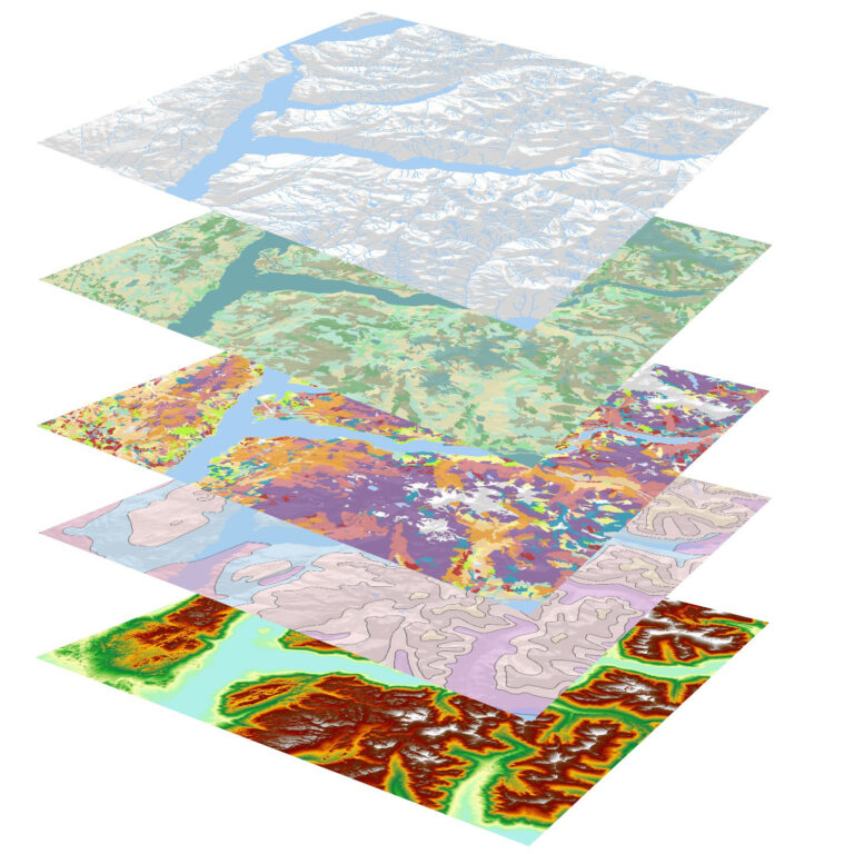
Overlay analysis combines multiple spatial layers to identify areas that simultaneously meet a set of criteria. It is one of the oldest and most widely used methods in GIS, and it sits at the heart of spatial decision-making workflows.

The underlying logic is straightforward.

You have a layer showing forest cover. Another showing slope. Another showing protected area boundaries. Overlay analysis lets you identify the areas that are forested, on slopes below 15 degrees, and outside protected boundaries. That location is a candidate zone for a specific land use decision.

Every layer adds a constraint, and the overlay operation finds where all constraints are satisfied simultaneously.

Common overlay operations include union (combining all features from two layers), intersection (keeping only the area where two layers overlap), and difference (removing the area of one layer from another).

In practice, overlay analysis is the backbone of land suitability modeling, environmental impact assessment, and site selection workflows across urban planning, conservation, and infrastructure development.

Proximity and Buffer Analysis

Proximity analysis measures spatial relationships based on distance.

Buffer analysis is its most common expression. It is creating a zone of a specified distance around a feature and using that zone to answer questions about what falls within or outside it.

For example, a 500-meter buffer around a school can identify all residences within walking distance for school zone planning. A 100-year flood zone buffer around a river system can identify which properties face inundation risk. A 15-minute drive-time buffer around emergency facilities can reveal which populations fall outside acceptable response time thresholds.

Buffer analysis is simple in concept but powerful in application. It translates abstract distance relationships into spatial zones that can be overlaid with other data layers to answer compound questions.

In my professional practice, proximity and buffer analysis are the methods I reach for first when a problem involves access, risk, or service delivery, because they translate spatial relationships directly into decision-relevant zones.

Network Analysis

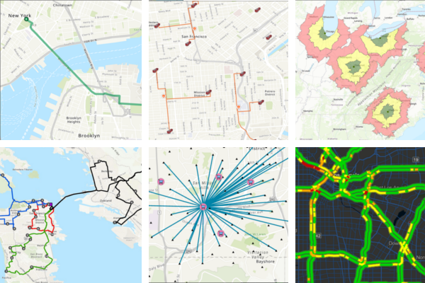
Network analysis examines movement and connectivity through spatial networks such as road systems, transit routes, river networks, and utility corridors.

Unlike straight-line proximity analysis, network analysis follows the actual paths along which movement occurs, making it the appropriate method for any question involving real-world travel or flow.

Core network analysis operations include:

• shortest path (finding the optimal route between two points),
• service area analysis (delineating the area reachable within a given time or distance from a facility), and
• origin-destination matrix generation (calculating travel costs between all combinations of origins and destinations in a dataset).

Applications are broad and practical.

Emergency response planners use network analysis to optimize ambulance station locations. Logistics companies use it to minimize delivery route distances. Urban planners use it to assess transit accessibility across a city. Retail analysts use it to measure catchment areas for store locations.

Any question that involves getting from somewhere to somewhere else through a network, under real constraints, is a network analysis problem.

Surface and 3D Analysis

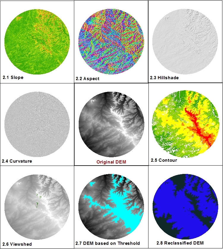
Surface analysis treats the landscape as a continuous three-dimensional form and extracts information about its shape, structure, and behavior. It is the primary analytical framework for working with elevation data: Digital Elevation Models (DEMs), Digital Surface Models (DSMs), and LiDAR-derived point clouds.

Core surface analysis operations include:

• slope calculation (measuring the rate of elevation change across a surface),
• aspect (determining the direction a slope faces, critical for solar radiation and vegetation modeling),
• hillshade (generating a simulated illumination of the terrain for visualization),
• viewshed analysis (identifying all areas visible from a given observer point), and
• watershed delineation (identifying the drainage basin that contributes flow to a specific outlet point).

3D analysis extends surface analysis into full three-dimensional space.

Building height and volume calculations from LiDAR or photogrammetric point clouds, solar potential modeling for urban rooftops, noise propagation modeling through three-dimensional urban environments, and line-of-sight analysis for telecommunications infrastructure planning all require 3D analytical capability that goes beyond what two-dimensional GIS operations can handle.

As I’ve found working with LiDAR datasets in urban and forested environments, surface and 3D analysis is where the true depth of geospatial data becomes apparent.

The landscape isn’t flat, and the analytical methods that respect its three-dimensional structure consistently produce more accurate and more useful outputs than their 2D equivalents.

Spatial Statistics

Spatial statistics quantifies patterns and relationships in geographic data. They are moving beyond visual interpretation to rigorous, testable measurements of how spatial phenomena are distributed and how they relate to each other.

Hotspot analysis identifies clusters of high or low values that are statistically significant, not just visually prominent.

Spatial autocorrelation measures whether similar values tend to cluster together in space (positive autocorrelation) or alternate randomly (no autocorrelation).

Kernel density estimation generates smooth, continuous surfaces from point data, revealing the underlying density of events across space.

Geographically weighted regression models how relationships between variables vary across a study area, allowing the analyst to see not just whether two variables are correlated, but where that correlation is strongest and where it breaks down.

These methods are essential in fields where the difference between a real spatial pattern and a random distribution matters — epidemiology, criminology, ecology, and social science.

From what I’ve seen in analytical practice, spatial statistics is consistently the most underused layer in geospatial workflows, even among experienced GIS users and adding it to a standard mapping analysis often produces the most genuinely surprising insights.

Change Detection and Temporal Analysis

Change detection analysis compares spatial data collected at different points in time to identify, map, and quantify what has changed — where, how much, and at what rate.

The most common application uses multitemporal satellite imagery to detect land cover change: forest loss, urban expansion, coastal erosion, wetland drainage, and agricultural conversion.

By comparing classified or spectral images from two or more dates, analysts can produce change maps that quantify transitions between land cover classes and calculate rates of change over time.

Temporal analysis extends this concept to any time-series spatial dataset.

Tracking the progressive expansion of an invasive species, monitoring the gradual subsidence of an urban area using InSAR data, or analyzing how pedestrian traffic patterns in a city shift across seasons are all temporal analysis problems.

The common thread is that time is treated as an analytical dimension alongside space, and change is the variable of interest.

Spatial Interpolation

Spatial interpolation estimates values at locations where no measurement exists, based on the values observed at surrounding measured points.

It is the method that turns a sparse network of weather stations into a continuous temperature surface, or a set of soil sample points into a map of organic matter content across a field.

The foundational principle is Tobler’s First Law of Geography: everything is related to everything else, but near things are more related than distant things.

Interpolation methods use this principle mathematically to weight surrounding observations by distance and generate estimates at unmeasured locations.

Common interpolation methods include Inverse Distance Weighting (IDW), which weights observations inversely proportional to their distance from the estimation point, and kriging, which uses a statistical model of spatial autocorrelation to produce both interpolated values and estimates of prediction uncertainty.

Kriging is the more sophisticated approach and is widely used in environmental monitoring, precision agriculture, hydrology, and climate science, where understanding the uncertainty of interpolated surfaces matters as much as the surfaces themselves.

What Tools Are Used for Geospatial Analysis?

The spatial analysis tool landscape is wide and growing. The right choice depends on your data volume, technical background, collaboration needs, and the specific methods your work requires.

Desktop GIS — QGIS and ArcGIS Pro

Desktop GIS platforms are the traditional home of geospatial analysis.

QGIS is the leading open-source option. It’s free, powerful, and supported by a large global community. It handles vector and raster analysis, spatial statistics, network analysis, and 3D visualization, and it integrates with Python for scripting and automation.

ArcGIS Pro is Esri’s professional desktop platform, the more polished, more deeply integrated with the broader ArcGIS ecosystem, and the standard in many government and enterprise environments, but requires a paid license.

Desktop GIS is the right choice for interactive, exploratory analysis where you want to see your data visually as you work with it: running queries, adjusting parameters, and iterating on outputs within a map-centric environment.

For cartographic production and final map output, desktop GIS remains the gold standard.

Cloud GIS — Google Earth Engine and ArcGIS Online

Cloud platforms bring the computation to the data rather than requiring you to download and process it locally.

Google Earth Engine provides access to petabytes of satellite imagery alongside a JavaScript and Python API for running large-scale raster analysis, including change detection across decades of Landsat imagery, global vegetation index time series, and continental flood mapping, at scales that desktop GIS cannot practically handle.

ArcGIS Online provides collaborative web-based analysis, hosted feature services, and a growing library of ready-to-run spatial analysis tools accessible through a browser.

Cloud GIS is the right choice when your data is too large for local processing, when collaboration across a team is required, or when you need to build analysis workflows that run automatically on new data as it arrives.

Programming — Python and R

Python and R give geospatial analysts the flexibility, reproducibility, and automation capability that GUI-based platforms cannot match.

Python’s geospatial ecosystem is particularly rich:

• GeoPandas handles vector data with a DataFrame interface familiar to any data analyst,
• Shapely provides computational geometry operations,
• Rasterio handles raster data,
• PySAL implements spatial statistics methods, and
• Folium and Plotly produce interactive web map outputs.

R’s sf package brings tidy spatial data workflows to the R ecosystem, with spdep for spatial statistics and tmap for visualization.

Programming-based workflows are the right choice for reproducible research, automated pipelines that run on scheduled data updates, custom analytical methods not available in GUI tools, and integration with broader data science and machine learning workflows.

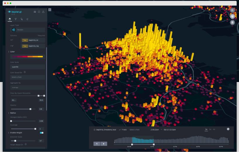
No-Code Platforms — CARTO, Felt, Kepler.gl

No-code platforms lower the barrier to spatial analysis for users who need spatial insights without the overhead of GIS software or programming.

• CARTO provides cloud-based spatial analytics with a visual interface and SQL-based data management.
• Felt enables collaborative browser-based mapping with data upload, styling, and basic spatial operations.
• Kepler.gl renders large point, line, and polygon datasets in the browser with no setup required: paste in a CSV with coordinates and explore.

These platforms are the right entry point for analysts coming from business intelligence, journalism, or general data analysis backgrounds who need to add a spatial dimension to their work without a steep learning curve.

What Does a Geospatial Analysis Workflow Look Like?

Understanding the individual methods and tools is important.

But geospatial analysis in practice always follows a workflow.

Here’s what that looks like end to end, using a hospital accessibility study as a concrete example.

Stage 1: Define the Question

Every analysis begins with a spatial question.

For this example, which residential areas in a city fall outside a 20-minute drive of the nearest emergency hospital?

A well-defined spatial question specifies the geographic extent of the analysis, the data layers required, the method appropriate to the question, and what the output needs to communicate to be useful.

Vague questions produce vague analyses. Precision here saves time at every subsequent stage.

Stage 2: Collect and Prepare the Data

Data preparation is consistently the most time-consuming stage of this process.

For the hospital accessibility study, you need a hospital locations layer, a road network dataset, a residential population layer, and an administrative boundary for the study area.

Each dataset needs to be checked for coordinate reference system consistency, attribute completeness, geometric validity, and temporal currency.

Reprojecting layers to a common CRS, clipping to the study area boundary, fixing invalid geometries, and resolving attribute inconsistencies all happen here before any analysis begins.

In my experience, analysts who rush this stage spend far more time debugging results than they saved by skipping it.

Stage 3: Perform the Analysis

With clean, consistent data, the analysis itself is often the fastest stage.

For the hospital accessibility study:

1. Run a drive-time service area analysis from each hospital location using the road network, set to a 20-minute threshold.
2. Overlay the resulting service area polygons with the residential population layer. Identify the residential areas that fall outside all service areas.
3. Calculate the population living in those areas.

The method follows directly from the question. The quality of the output depends almost entirely on the quality of the data preparation that preceded it.

Stage 4: Validate and Interpret Results

Raw analytical outputs always require validation before interpretation.

Check whether the service area boundaries follow the road network realistically. Verify that population estimates match known totals. Identify any areas that appear anomalous and trace them back to potential data issues.

Interpretation goes beyond the numbers.

• What do the results mean in the context of the city’s geography, demographics, and existing health infrastructure?
• Are the underserved areas concentrated in particular neighborhoods?
• Do they correlate with other indicators of socioeconomic disadvantage?

This is where spatial analysis becomes spatial understanding.

Stage 5: Communicate the Output

The final stage is making the results accessible to the people who need to act on them.

For the hospital accessibility study, this might mean a map showing the underserved zones overlaid on a population density basemap, a summary table of affected population by neighborhood, and a set of scenario outputs showing how a new hospital at different candidate locations would change the coverage picture.

Effective communication of analysis results requires both cartography skills to make a map that is clear, accurate, and honest, and analytical literacy to present uncertainty, limitations, and caveats alongside the headline findings.

Where Is Geospatial Analysis Applied?

Geospatial analysis supports decision-making across virtually every field that involves the Earth’s surface. The applications article in this series covers the full landscape in depth, but here is a brief orientation to the six most significant domains.

• Environmental monitoring and conservation use spatial analysis to track ecosystem change, model species habitat, assess land degradation, and prioritize conservation interventions.
• Urban planning and infrastructure rely on spatial analysis for land use zoning, infrastructure siting, accessibility assessment, and growth management.
• Public health and epidemiology use proximity, network, and statistical analysis to map disease distribution, identify exposure risks, and plan health service delivery.
• Agriculture and food security apply spatial analysis to crop monitoring, yield modeling, soil characterization, and irrigation management.
• Disaster risk and emergency management use it for flood zone delineation, evacuation route planning, damage assessment, and early warning system design.
• Business and location intelligence apply spatial analysis to retail site selection, market area delineation, logistics optimization, and customer catchment modeling.

How Do You Start Practicing Geospatial Analysis?

The most effective way to learn spatial analysis is to run a real analysis on a real dataset, not to read about it.

Here are three entry points matched to different starting points.

Beginner: Buffer and overlay analysis in QGIS

• Download QGIS free at qgis.org.
• Load a point dataset — hospital locations, school locations, or any point layer for your area of interest from OpenStreetMap.
• Run a buffer operation at a distance relevant to your question.
• Overlay the buffer zones with a polygon layer — neighborhood boundaries, land parcels, or a population grid.
• Explore what the intersection reveals.

Intermediate: Hotspot analysis in QGIS or ArcGIS Online

1. Download a point event dataset — crime incidents, disease cases, species observations — for a city or region of interest.
2. Run a kernel density estimation to visualize event density across space.
3. Then run a Getis-Ord Gi* hotspot analysis to identify statistically significant clusters.
4. Compare what the density map shows versus what the statistical hotspot analysis reveals.

Advanced: Spatial analysis workflow in Python

1. Install GeoPandas, Shapely, and PySAL in a Python environment.
2. Load a vector dataset with GeoPandas.
3. Run a buffer, perform a spatial join, calculate area statistics by polygon, and visualize the output with Folium.
4. Then extend the workflow by adding a spatial weights matrix with PySAL and running a Moran’s I spatial autocorrelation test on a numeric attribute.

Wrap Up

Geospatial analysis is what transforms location data from a coordinate into a decision.

The methods range from simple proximity queries to complex predictive models, but the underlying logic is consistent: location matters, spatial relationships reveal patterns that non-spatial analysis misses, and those patterns have real consequences for how we plan, allocate, respond, and design.

The seven core analysis types (overlay, proximity and buffer, network, spatial statistics, change detection, spatial interpolation, and surface and 3D analysis) cover the analytical vocabulary you need to work across the full range of geospatial problems.

The tools are largely free or accessible. The workflows are learnable. And the field rewards practice more than theory.

The best geospatial analysis you’ll ever do is the next one.

Start with a question that matters to you, find the data, and run the analysis.

Get out there and run the analysis.

FAQ

What is geospatial analysis in simple terms?

Geospatial analysis is the process of examining spatial data to find patterns, relationships, and insights that are defined by location. It goes beyond making maps — it uses analytical methods to answer questions about why things are where they are, how geographic features relate to each other, and what spatial patterns reveal about real-world phenomena. The output is not just a map but actionable knowledge grounded in location.

What is the difference between geospatial analysis and spatial analysis?

Spatial analysis is the broader, older term used in mathematics, statistics, and academic geography to describe any analytical method that incorporates position or space. Geospatial analysis refers specifically to spatial analysis applied to Earth’s surface, using GIS tools, remote sensing data, and geographic coordinate systems. In professional GIS and Earth observation contexts, spatial analysis is the standard term — spatial analysis appears frequently as a synonym and is used throughout the field.

What are the main types of geospatial analysis?

The seven core types of geospatial analysis are overlay analysis (combining layers to identify areas meeting multiple criteria), proximity and buffer analysis (measuring distance relationships), network analysis (analyzing movement through spatial networks), spatial statistics (quantifying spatial patterns and relationships), change detection (comparing spatial data across time), spatial interpolation (estimating values at unmeasured locations), and surface and 3D analysis (analyzing terrain structure and three-dimensional spatial relationships).

What tools are used for geospatial analysis?

Geospatial analysis tools span four categories. Desktop GIS platforms — QGIS (free) and ArcGIS Pro — support interactive analysis and cartographic output. Cloud platforms — Google Earth Engine and ArcGIS Online — enable large-scale processing and collaboration. Programming environments — Python with GeoPandas and PySAL, and R with sf and spdep — support reproducible and automated workflows. No-code platforms — CARTO, Felt, and Kepler.gl — provide accessible entry points for analysts without GIS software experience.

What is overlay analysis in GIS?

Overlay analysis combines two or more spatial layers to identify areas that simultaneously meet a set of criteria. It works by superimposing layers and performing operations — union, intersection, or difference — to create new features that reflect the combined spatial and attribute properties of the input layers. Overlay analysis is widely used in land suitability modeling, environmental impact assessment, and site selection workflows.

How do I get started with geospatial analysis?

The most effective starting point depends on your background. If you’re new to GIS, download QGIS and run a buffer and overlay analysis on a free dataset from OpenStreetMap or Natural Earth. If you’re a data analyst comfortable with Python, install GeoPandas and run a spatial join and buffer workflow on a dataset relevant to your field. If you prefer no-code tools, upload a CSV with coordinates to Kepler.gl and explore the spatial distribution of your data visually. In every case, start with a real question and real data — not a tutorial dataset.

Take Your Analysis Further

Geospatial analysis is the core skill of the geospatial field.

The next level beyond analysis is geospatial modeling: building spatial representations that simulate processes, predict outcomes, and test scenarios before committing to real-world decisions.

The geospatial modeling article covers what spatial models are, how they’re built, and where they’re applied, from hydrological flow models to urban growth simulations to predictive habitat models. It’s the natural next step for anyone who has worked through the analysis methods covered here.

If you’re working through a specific analysis problem — choosing the right method, finding the right data, or interpreting unexpected results — drop a comment below. Let’s work through it together.

Happy mapping!