Overlay Analysis in GIS: How Combining Geospatial Layers Reveals What Maps Alone Cannot

What is overlay analysis in GIS? Learn how vector overlay, raster overlay, and weighted overlay work — with types, examples, applications, and a step-by-step workflow.

A parcel of land exists simultaneously inside a flood zone, outside a protected area boundary, within a specific school district, and adjacent to a transit corridor.

None of those layers was created with the others in mind.

The flood zone boundary came from a hydraulic model. The protected area boundary came from a conservation agency. The school district boundary came from a local education authority. The transit corridor came from a transportation planner.

Overlay analysis is the GIS operation that combines them — superimposing multiple spatial layers to create a single analytical output that reflects the combined attributes and spatial relationships of all inputs simultaneously.

It is what makes GIS more than a digital map.

A digital map shows you where things are. Overlay analysis shows you what multiple spatial realities, stacked in the same place, add up to.

What Is Overlay Analysis in GIS?

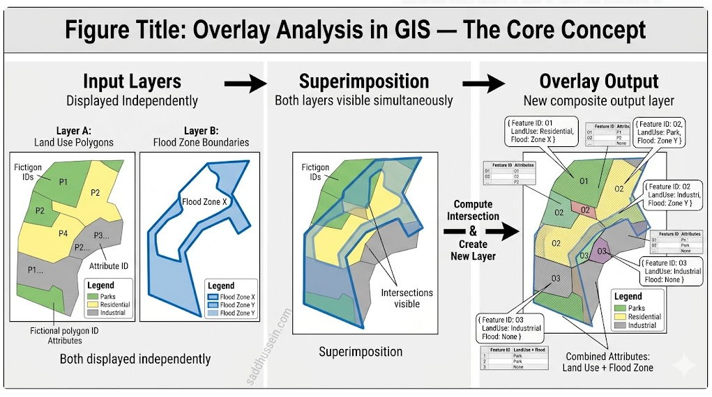
Overlay analysis is the operation of superimposing two or more geospatial layers to create a new layer that combines their geometric boundaries and attribute information.

Where the boundaries of input layers intersect, new feature boundaries are created in the output. Where features from different layers occupy the same space, their attributes are combined in the output feature record.

The concept predates digital GIS by decades.

Ian McHarg’s 1969 book Design with Nature described a manual overlay process — drawing environmental, social, and physical data on transparent acetate sheets and physically stacking them to identify areas of combined suitability or constraint.

Each sheet represented one spatial variable. The stack represented the interaction of all variables simultaneously. GIS digitized and automated that process, adding computational precision, quantitative attribute combination, and the ability to work with layers at scales and with complexity that acetate sheets could not handle.

Overlay analysis is not a single operation.

It is a family of operations, divided primarily into vector and raster implementations, each with distinct subtypes appropriate for different analytical purposes.

Understanding which overlay operation to use, and when, is one of the core analytical competencies in GIS practice.

The unifying principle across all overlay types is the same: spatial location is the join key.

In database terms, overlay analysis is a spatial join that creates new records wherever input geometries intersect — but unlike a standard attribute join keyed on a shared field value, an overlay join is keyed on shared geographic space.

Features are related not because they share an ID but because they occupy the same location.

What Are the Types of Vector Overlay Analysis?

Vector overlay analysis operates on discrete geographic features — polygons, lines, and points — and produces new feature geometries defined by the intersections of the input layer boundaries.

The choice between vector overlay types determines which parts of the input features appear in the output and how their attributes are combined.

Intersect

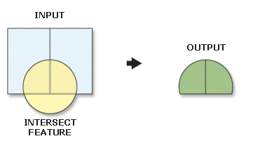
Intersect is the most widely used vector overlay operation. The output contains only the features — or portions of features — that fall within the spatial extent shared by all input layers. Features entirely outside the overlap area are excluded from the output.

The geometric result of an intersect depends on the input feature types:

• polygon-on-polygon intersect produces output polygons at every intersection of input boundaries;
• line-on-polygon intersect produces line segments clipped to polygon boundaries with polygon attributes attached;
• point-in-polygon intersect produces only the points that fall within the overlay polygon layer, with polygon attributes joined.

The analytical utility of intersect is the question it answers:

• what attributes from Layer B apply to features in Layer A, and
• what is the geometry of the overlap? .

A parcel layer intersected with a flood zone layer produces an output containing only the portions of parcels within the flood zone, with both parcel attributes and flood zone attributes on each output feature — the spatial foundation for flood exposure analysis, insurance risk assessment, and regulatory compliance checking.

Union

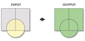
Union combines all features from all input layers into a single output, preserving the complete spatial extent of every input, not just the overlap.

Where features from different layers occupy the same space, the output inherits attributes from all relevant inputs. Where features from one layer have no corresponding overlap with another, the output records null values for the attributes of the absent layer.

Union is the most attribute-rich overlay output and the most analytically complex to work with.

A union of three polygon layers produces an output where every polygon records attributes from all three inputs, with null values wherever a given location fell outside the extent of one input.

The output polygon count is typically much larger than any input. Every intersection of every boundary from every input layer creates a new output polygon boundary.

Union is appropriate when the analysis requires the complete spatial record of all input layer features, not just their overlap.

A land use planning analysis combining zoning, ownership, and infrastructure proximity layers may require union to preserve all parcels even those outside infrastructure corridors — so that the full planning area is covered in the output.

Clip

Clip uses one layer — the clip feature — as a geographic cookie cutter applied to another layer — the input feature.

The output contains only the portions of the input features that fall within the clip feature boundary. No attribute combination occurs as the output retains only the attributes of the input layer, not the clip layer.

Clip is technically an overlay operation, but analytically it functions as a geographic filter rather than an attribute combination.

It is the appropriate operation when the goal is to reduce the spatial extent of a layer to a specific study area boundary, i.e.,

• clipping a national road network to a county boundary,
• clipping a global species distribution model to a protected area polygon, or
• clipping a land cover raster to a watershed boundary before further analysis.

The distinction between clip and intersect is important: clip preserves only input layer attributes within the clip boundary.

Intersect preserves attributes from both input layers within their shared boundary. When an attribute combination is needed, intersect is correct. When geographic subsetting without attribute combination is needed, the clip is correct.

Erase

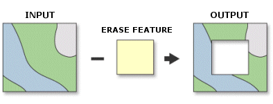
Erase is the inverse of clip — the output contains the portions of the input layer that fall outside the erase feature boundary.

Features within the erase boundary are removed from the output. Like clip, erase is a geometric filtering operation that does not combine attributes.

Erase is appropriate for removing exclusion zones from an analysis area, for example:

• erasing protected areas from a development suitability surface,
• erasing existing built-up areas from a greenfield development analysis, or
• erasing flood zone polygons from an agricultural suitability layer to exclude flood-prone land from the output.

Identity

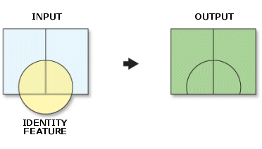
Identity preserves all features of one designated layer — the identity layer — in the output, while overlaying it with a second layer.

Features in the identity layer that fall within the overlay layer acquire the overlay layer’s attributes. Features in the identity layer that fall outside the overlay layer are preserved in the output with null values for the overlay attributes.

Identity is the appropriate operation when preserving the complete spatial coverage of one layer is required, while enriching it with attributes from a second layer where the two overlap.

A parcel layer enriched with school district attributes uses identity — every parcel is preserved in the output, acquiring the school district attribute where the parcel falls within a district boundary and null where no district data exists.

Symmetrical Difference

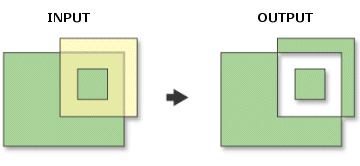
Symmetrical difference produces an output containing the features from each input layer that do not overlap with the other.

The shared overlap area is excluded.

The result is the spatial equivalent of the exclusive OR logical operation — features that are in one layer or the other but not both.

Symmetrical difference is the least commonly used of the standard vector overlay operations, but analytically valuable for change detection, especially for identifying the areas that were in a previous land cover classification but are absent from a current one (loss), and the areas present in the current classification but absent from the previous (gain), excluding the unchanged areas common to both.

What Is Raster Overlay Analysis?

Raster overlay analysis operates on grid-based geospatial data.

It applies mathematical or logical operations to corresponding cells across multiple raster layers to produce an output raster where each cell value reflects the combined conditions of all input layers at that location.

Map Algebra — The Foundation of Raster Overlay

Map algebra is the mathematical framework for raster overlay, by treating each raster layer as a variable in an equation and performing cell-by-cell calculations across the entire spatial extent.

Esri introduced the term in the 1980s through Dana Tomlin’s work on cartographic modeling, and it remains the conceptual foundation of raster overlay analysis in every GIS platform.

Map algebra operations fall into four categories.

Local operations calculate output cell values from the corresponding cells of multiple input rasters — addition, subtraction, multiplication, and logical operations are all local operations. The NDVI vegetation index calculation — (NIR – Red) / (NIR + Red) — is a local map algebra operation on two satellite imagery bands.

Focal operations calculate output cell values from a neighborhood of cells surrounding each cell — slope calculation from a DEM is a focal operation using a 3×3 cell neighborhood.

Zonal operations calculate statistics for all cells within defined zones — calculating mean elevation within each watershed polygon is a zonal operation.

Global operations use the entire raster extent in the calculation — Euclidean distance surfaces are global operations.

Reclassification Before Overlay

Raster overlay analysis almost always requires reclassification before combination.

It convert raw input raster values to a common scale that makes meaningful addition or comparison possible.

A slope raster measured in degrees and a precipitation raster measured in millimeters cannot be meaningfully added as raw values.

Reclassifying both to a 1-5 or 1-9 suitability scale — where 1 represents least suitable and 5 or 9 represents most suitable for the analysis purpose — converts heterogeneous inputs to a common analytical currency.

Reclassification assigns new values to ranges of existing values based on their relevance to the analytical objective.

For a crop suitability analysis, slopes between 0 and 2 degrees might be reclassified as 5 (most suitable), slopes between 2 and 5 degrees as 4, between 5 and 10 degrees as 3, between 10 and 15 degrees as 2, and above 15 degrees as 1 (least suitable).

The reclassification scheme embeds the domain knowledge about what conditions favor the analytical objective, and making it one of the most important and judgment-dependent steps in the overlay workflow.

Boolean Overlay Operations

Boolean overlay applies logical operations — AND, OR, NOT, XOR — to binary raster inputs where cell values represent the presence or absence of a condition.

For example, a flood zone raster (1 = in flood zone, 0 = outside) AND a steep slope raster (1 = slope above 15 degrees, 0 = slope below 15 degrees) produces a raster where cells with value 1 are simultaneously in the flood zone and on steep slope. The spatial intersection of both constraints expressed as a Boolean combination.

Boolean overlay is the raster equivalent of vector intersect, as it identifies locations where multiple binary conditions are simultaneously true.

It is the appropriate approach when the analysis requires a hard constraint — locations must meet all criteria to be included, with no partial credit for meeting only some.

What Is Weighted Overlay Analysis?

Weighted overlay analysis is a suitability modeling framework.

It is a structured approach to combining multiple spatial criteria into a composite suitability surface that ranks every location by its overall suitability for a defined purpose.

It is the most analytically sophisticated form of raster overlay and the standard methodology for spatial decision support.

The Weighted Overlay Framework

The weighted overlay process follows a structured sequence.

Each input criterion is represented as a raster layer. Each layer is reclassified to a common suitability scale — typically 1 to 9, where 9 represents the most suitable conditions and 1 the least.

Each reclassified layer is assigned a percentage weight reflecting its relative importance to the overall suitability judgment.

The weighted layers are summed — each cell’s output value is the sum of its reclassified values across all input layers, each multiplied by its weight — producing a continuous suitability surface across the analysis area.

The mathematical formulation is straightforward.

If three criteria — soil quality (weight 50%), slope (weight 30%), and distance to water (weight 20%) — are combined, the suitability score at any location is: (soil quality reclassified value × 0.50) + (slope reclassified value × 0.30) + (distance to water reclassified value × 0.20).

Every location in the study area receives a suitability score reflecting its combined performance across all weighted criteria.

Weight Assignment and Domain Knowledge

Weight assignment is where analytical judgment and domain knowledge most directly shape the output.

The weights encode the relative importance of each criterion — and different weight assignments produce different suitability surfaces from the same input data.

A conservation planner might weight habitat connectivity at 40 percent and human disturbance at 30 percent.

A developer evaluating the same landscape might weight accessibility at 40 percent and slope at 30 percent. Same layers, same reclassification scales, different weights — different outputs, different spatial priorities.

From my experience working with weighted overlay in planning and environmental contexts, the weight assignment step benefits most from explicit stakeholder engagement and sensitivity analysis.

Weights should reflect the values and priorities of the decision-making process and not just the analyst’s default assumptions.

And sensitivity analysis (running the model with alternative weight sets and comparing how much the output changes) quantifies how dependent the suitability ranking is on the weight choices, revealing whether the top-ranked locations are robust across a range of weight assumptions or sensitive to specific weighting decisions.

Multi-Criteria Evaluation and Constraints

Weighted overlay is a form of multi-criteria evaluation.

It is a decision-support methodology that combines multiple criteria into a single composite score to support spatially explicit decision-making.

Hard constraints — areas that are categorically excluded regardless of their performance on other criteria — are handled by Boolean masking before or after the weighted overlay, not by low weights.

A protected area exclusion zone, a flood plain restriction, or a slope threshold above which development is infeasible should be applied as a hard constraint mask, not assigned a weight of 5 percent in the overlay.

Low weights allow constrained areas to still appear in the output with low scores; hard masks exclude them entirely. The distinction matters when output scores are used to rank sites for investment.

How Does Overlay Analysis Differ From Other GIS Operations?

Understanding when overlay analysis is the right tool requires distinguishing it from the related GIS operations that share surface similarity but serve different analytical purposes.

Overlay vs Spatial Join

A spatial join transfers attributes from one layer to another based on their spatial relationship, without creating new geometry.

A point layer of weather stations spatially joined to a polygon layer of climate zones acquires the climate zone attribute for each station point, but the point geometry is unchanged.

An overlay operation, by contrast, creates new geometry at the intersections of input layer boundaries; the output features are geometrically different from any input.

Use spatial join when the goal is attribute transfer without geometry modification.

Use overlay when the goal is both attribute combination and new geometry creation at layer intersections.

Overlay vs Buffer Analysis

Buffer analysis creates geometric zones of defined distance around features — a 500-meter buffer around a school, a 100-year flood buffer around a river channel.

It produces a new geometry layer representing proximity. Meanwhile, overlay analysis combines existing layers by superimposition — it does not create new proximity geometry; it combines what already exists.

In practice, buffer analysis frequently precedes overlay analysis: a 500-meter school buffer layer is created, then intersected with a rezoning application layer to identify which rezoning proposals fall within the school buffer.

The buffer creates the proximity feature; the overlay combines it with the application layer. They are complementary operations in a multi-step workflow, not alternatives to each other.

Overlay vs Clip

Clip is technically an overlay operation — it uses one layer’s geometry to define the spatial extent of an output derived from another layer.

But analytically, clip is a geographic subsetting tool, not a multi-criteria combination tool. Clip produces an output with the attributes of one layer only, geographically restricted to the extent of another. Overlay combines the attributes of both.

The practical test: if the analysis requires knowing which layer the output feature came from and what its attributes are — use intersect or union.

If the analysis simply needs to restrict one layer to a geographic boundary — use clip.

What Are the Real-World Applications of Overlay Analysis?

Overlay analysis is the analytical backbone of most GIS-based spatial decision support — appearing explicitly or implicitly in almost every domain where multiple spatial criteria inform a decision.

Land Use Suitability Analysis

Land use suitability analysis is the canonical weighted overlay application by combining soil quality, slope, distance to infrastructure, climate suitability, land tenure, and environmental constraint layers into a composite suitability surface that identifies the locations best suited for agriculture, residential development, industrial use, or conservation.

FAO’s land evaluation framework, the urban planning suitability models used by local authorities, and the agricultural investment suitability analyses used by development finance institutions all implement this logic — multiple criteria reclassified, weighted by importance, and combined into a spatial ranking.

Environmental Impact Assessment

Environmental impact assessment uses overlay analysis to define the spatial extent of project impacts and characterize the environmental resources within them.

The impact zone — usually defined by buffer analysis — is overlaid with layers of sensitive habitats, species occurrence, hydrological features, and land use to identify what environmental resources fall within the zone of potential impact.

Cumulative impact assessment overlays multiple project impact zones against each other and against sensitive receptor layers to identify geographic concentrations of combined impact.

Emergency Management

Hazard exposure mapping overlays flood zone, earthquake, and wildfire risk surfaces with population distribution, critical infrastructure locations, and social vulnerability indices to identify the communities and facilities facing the highest compound risk from multiple concurrent hazards.

The compound vulnerability maps used in disaster preparedness planning are weighted overlay outputs — multiple hazard and vulnerability layers combined into a spatial risk ranking that directs preparedness investment.

Urban Planning

Zoning compliance analysis overlays parcel boundaries with zoning district maps to identify parcels whose current use is non-conforming with their zoning designation.

Development constraint analysis overlays regulatory buffers, environmental protections, infrastructure easements, and slope limitations to identify the buildable area within a candidate development site.

Both are intersect overlay operations that combine the geometry and attributes of planning layers to answer specific regulatory questions.

What Are Common Errors and Limitations in Overlay Analysis?

Overlay analysis is powerful — and it amplifies the errors in its inputs as readily as it amplifies the insights.

Sliver Polygons

Sliver polygons are the most common artifact of vector overlay analysis.

Sliver polygons are thin, narrow polygon features created when two input layers contain boundaries that should be coincident but are slightly misaligned due to different source data, digitization methods, or coordinate systems.

When two layers that nominally share a boundary — a county line in a land use layer and the same county line in a census layer — are overlaid, small positional discrepancies produce thin slivers of erroneous output polygons along the shared boundary.

Slivers inflate the output feature count, introduce false area calculations, and complicate downstream analysis. Snapping input boundaries to each other before overlay, or applying a post-overlay minimum area threshold to remove tiny polygons, are the standard remedies.

Scale Mismatch

Overlay analysis combining layers created at different source scales produces outputs whose spatial precision is limited by the least precise input.

A flood zone boundary digitized at 1:100,000 scale combined with a parcel boundary digitized at 1:1,200 scale produces an output that appears to have parcel-level precision but whose flood zone boundary has 100-meter positional uncertainty.

The false precision of the output — appearing in detailed parcel geometry despite the coarse flood boundary — can mislead analysts into over-interpreting the overlay result.

Documenting and communicating the scale limitations of input layers is a professional obligation in overlay analysis, not a footnote.

Attribute Field Proliferation

Union overlay combines all attributes from all input layers in the output — which rapidly produces output feature classes with dozens of fields when multiple layers are combined.

Many of those fields will contain null values for features outside the extent of their source layer.

Managing the output attribute table is an unglamorous but essential step in producing a usable overlay output. It might include:

• removing irrelevant fields,
• renaming ambiguous fields from different source layers that share common field names, and
• documenting field provenance.

Data Quality Dependency

Overlay analysis inherits the positional errors, classification errors, and currency limitations of every input layer it combines.

An overlay output is only as reliable as its least reliable input. A weighted suitability analysis combining a current high-resolution soil survey with a decade-old land cover classification and a coarse-resolution climate interpolation produces a suitability surface whose reliability varies spatially with the currency and precision of the underlying data.

Explicit data quality assessment of each input layer before overlay, and transparent communication of data quality limitations in output products, is the methodological standard that separates defensible overlay analysis from superficially convincing but technically unreliable output.

A Complete GIS Workflow — Land Suitability Analysis Using Weighted Overlay

Weighted overlay suitability analysis is one of the most complete expressions of overlay analysis in practice — combining multiple criteria into a spatially explicit recommendation that directly supports a location decision.

Here is a complete workflow for agricultural land suitability analysis.

Step 1 — Define the objective and criteria.

The analysis objective: identify the land most suitable for rain-fed smallholder agriculture in a study region.

Criteria selected based on agronomic domain knowledge:

• soil texture and drainage (most important),
• annual rainfall (important),
• slope (important),
• distance to markets (moderate importance), and
• existing land cover — excluding forests and protected areas as hard constraints.

Step 2 — Assemble input raster layers.

Collect or derive raster layers for each criterion:

• soil texture and drainage class from the national soil survey data,
• annual rainfall from interpolated climate station data,
• slope derived from DEM using focal slope calculation,
• distance to markets calculated as Euclidean distance from market point locations, and
• land cover classification from Sentinel-2 satellite imagery.

Reproject all layers to a common equal-area CRS.

Resample all layers to the same cell size using the coarsest input resolution to avoid false precision in the output.

Step 3 — Apply hard constraint mask.

Create a binary mask raster where protected areas and forest cover cells are coded 0 (excluded) and all other cells are coded 1 (eligible).

This mask will be applied to the final suitability output to remove ineligible areas regardless of their suitability score.

Step 4 — Reclassify each criterion layer.

Reclassify each input layer from its raw values to a 1-9 suitability scale based on agronomic knowledge:

• well-drained loam soils reclassified as 9, poorly drained clays as 2;
• rainfall above 800mm as 9, below 400mm as 1;
• slopes below 2 degrees as 9, above 15 degrees as 1;
• distance to market below 10km as 9, above 50km as 2;
• and so on for each criterion.

Step 5 — Assign weights.

Based on domain knowledge and stakeholder consultation:

• soil quality 35%,
• annual rainfall 30%,
• slope 20%,
• distance to markets 15%.

Weights sum to 100 percent.

Step 6 — Run weighted overlay.

Multiply each reclassified layer by its weight and sum across all layers:

(soil × 0.35) + (rainfall × 0.30) + (slope × 0.20) + (market distance × 0.15).

The output is a continuous suitability surface with values ranging from approximately 1 (least suitable) to 9 (most suitable).

Step 7 — Apply constraint mask.

Multiply the suitability surface by the constraint mask — setting protected area and forest cells to NoData. The final output shows suitability scores only for eligible land.

Step 8 — Classify and interpret output.

Reclassify the final suitability surface into discrete classes for communication to decision-makers and stakeholders:

• highly suitable (7-9),
• moderately suitable (4-6),
• marginally suitable (2-3),
• not suitable (1)

Calculate the area in each class by administrative unit.

Step 9 — Sensitivity analysis.

Run the model with alternative weight sets (i.e., increasing soil weight to 50% and reducing rainfall weight to 20%) and compare how the top-ranked areas change.

Areas that rank highly across multiple weight configurations are more robust recommendations than areas that only rank highly under one specific weight assumption.

The output is a spatially explicit, analytically transparent suitability ranking that supports agricultural investment prioritization, extension service targeting, and land use planning.

It is complemented by a documented methodology that can be audited, updated as new data becomes available, and adapted to different crop types or management systems by adjusting the reclassification schemes and weights.

Wrap Up

Overlay analysis is not just a GIS operation.

It is the spatial embodiment of a question that most spatial decisions require answering: what do multiple realities, stacked in the same place, add up to?

A parcel is simultaneously in a flood zone, outside a protected area, within a school district, and along a transit corridor.

A landscape cell is simultaneously suitable soil, gentle slope, adequate rainfall, and accessible to markets.

A neighborhood is simultaneously high hazard, high vulnerability, and low service coverage.

None of those conditions is the full story. All of them together are.

Overlay analysis is how GIS answers questions that no single layer can answer alone by combining the evidence that spatial decisions require into outputs that reflect the world’s real complexity rather than the convenient simplicity of one map at a time.

FAQ

What is overlay analysis in GIS?

Overlay analysis is the GIS operation of superimposing two or more spatial layers to create a new layer that combines their geometric boundaries and attribute information. Where input layer boundaries intersect, new feature boundaries are created in the output. Where features from different layers occupy the same space, their attributes are combined. Overlay analysis is the foundational multi-criteria spatial reasoning operation in GIS — enabling analysts to ask questions that no single layer can answer by combining multiple spatial realities into a single composite output. It exists in both vector form (operating on discrete features) and raster form (operating cell by cell on grid data).

What are the types of overlay analysis in GIS?

Vector overlay analysis has six main types. Intersect produces output containing only features within the spatial overlap of all input layers. Union produces output containing all features from all input layers, combining attributes where layers overlap. Clip uses one layer as a geographic boundary to extract the corresponding portions of another layer without attribute combination. Erase removes the area of one layer from another, producing the input layer minus the erase layer. Identity preserves all features of one designated layer while adding attributes from a second where they overlap. Symmetrical difference produces features present in one layer but not the other, excluding the shared overlap. Raster overlay analysis uses map algebra — local, focal, zonal, and global operations — to combine cell values across multiple raster grids.

What is the difference between union and intersect in GIS?

Intersect produces an output containing only the features or portions of features that fall within the spatial overlap of all input layers — features entirely outside the shared area are excluded. Union produces an output containing all features from all input layers — those within the shared overlap acquire combined attributes from both layers, while those outside the overlap retain their own attributes with null values for the absent layer’s attributes. Intersect answers “what is common to all layers?” Union answers “what is the complete spatial record of all layers combined?” Intersect produces a smaller, more focused output. Union produces a complete but more complex output with many null attribute values for non-overlapping features.

What is weighted overlay analysis in GIS?

Weighted overlay analysis is a suitability modeling framework that combines multiple spatial criteria into a composite suitability surface. The process involves four steps: reclassifying each input raster layer from its raw values to a common suitability scale (typically 1-9); assigning percentage weights to each layer reflecting its relative importance; multiplying each reclassified layer by its weight; and summing the weighted layers to produce a composite suitability score for every cell in the analysis area. The result is a continuous surface ranking locations by their overall suitability for a defined purpose — used in agricultural land evaluation, conservation prioritization, urban development planning, and any spatial decision requiring the combination of multiple criteria with different levels of importance.

What is the difference between vector and raster overlay analysis?

Vector overlay analysis operates on discrete geographic features — polygons, lines, and points — and creates new feature geometries at the intersections of input layer boundaries. It preserves topological relationships between features and produces exact geometric outputs with combined attribute tables. Raster overlay analysis operates cell by cell on grid data — applying mathematical or logical operations to corresponding cells across multiple raster grids simultaneously. It is more efficient for continuous spatial phenomena, supports mathematical operations that vector overlay cannot perform, and is the standard approach for suitability modeling. Vector overlay is preferred when precise feature boundaries and complete attribute information matter. Raster overlay is preferred when continuous surfaces, map algebra operations, and weighted suitability analysis are required.

What are common applications of overlay analysis in GIS?

Overlay analysis is the core analytical operation in spatial suitability modeling — agricultural land evaluation, urban development suitability, conservation priority mapping, and site selection all use weighted overlay to combine multiple criteria into composite rankings. Environmental impact assessment uses intersect overlay to identify the environmental resources within project impact zones. Emergency management uses weighted overlay to map compound hazard and vulnerability exposure. Urban planning uses overlay to identify zoning non-conformities, development constraints, and infrastructure service gaps. Conservation planning uses overlay to identify gaps in protected area coverage relative to biodiversity distribution. Any GIS analysis requiring the combination of multiple spatial layers to answer a question that no single layer can answer alone uses overlay analysis as its foundational operation.

What’s Next

Overlay analysis answers what multiple spatial realities, stacked in the same place, add up to. Proximity analysis answers a different but equally fundamental spatial question: how far is it, and does distance matter?

The next article in the geospatial analysis series covers proximity analysis, such as buffers, distance surfaces, nearest neighbor analysis, and the spatial operations that make distance a rigorous analytical variable in GIS.

Questions about overlay analysis — vector overlay operations, weighted suitability modeling, map algebra, or dealing with sliver polygons — drop them in the comments. Let’s work through it together.

Happy mapping!