Learn what cost distance analysis in GIS is, how resistance surfaces and accumulated cost work, and how least cost path analysis finds wildlife corridors.
Two wildlife habitat patches sit 5 kilometers apart on a map.
By straight-line distance, they are close. But between them lies a mosaic of agricultural fields, a four-lane highway, and a stretch of industrial land on the edge of a city.
For a forest-dependent species attempting to disperse between the patches, that 5-kilometer gap might as well be impassable.
The question is not how far the patches are from each other.
The question is whether anything can move between them, and if so, through what route.
That is the question cost distance analysis in GIS was built to answer.
Contents
What Is Cost Distance Analysis in GIS?
Cost distance analysis generalizes the concept of distance to account for the variable effort of moving across a landscape.
Instead of asking how far two locations are from each other in straight-line terms, it asks:
What is the total accumulated cost of traveling from a source to a destination through the path of least resistance, given that some parts of the landscape are easy to traverse and others are close to impassable?
The output is not a single number.
It is a surface: a raster grid where every cell holds the minimum total travel cost from the source location to that cell, calculated by routing through the landscape rather than drawing a straight line across it.
Think of it as the difference between measuring the distance across a city on a flat map and measuring the actual effort of a hike through mountainous terrain.
The map distance tells you where things are.
The accumulated cost surface tells you what it costs to get there through a specific environment, given a specific kind of movement.
How Cost Distance Differs from Euclidean and Network Distance
The three main distance concepts in proximity analysis each assume something different about how movement works.
Euclidean distance assumes movement is unconstrained and equal in all directions: a signal radiates, a setback zone expands, a buffer circle grows outward uniformly.
Network distance assumes movement follows a discrete infrastructure system: roads, paths, utility lines.
Cost distance assumes movement crosses a continuous landscape where resistance varies cell by cell, and the traveler takes whatever route minimizes the total accumulated effort.
Wildlife dispersal belongs in the cost distance category.
A lynx moving between forest patches does not follow roads. It moves through the terrain, finding the routes where forest cover is continuous, slopes are manageable, and human disturbance is low.
A road network dataset is useless for modeling that movement. A Euclidean distance is misleading. A resistance surface and an accumulated cost model is the right tool.
So is overland water flow, emergency evacuation through partially damaged infrastructure, and off-road military movement planning.
Wherever movement crosses a continuous surface with spatially variable friction, cost distance analysis is the appropriate method.
What Is a Cost Raster in GIS?
The cost raster is the foundation of cost distance analysis. Without it, there is no analysis.
A cost raster is a raster layer where each cell value represents the resistance or friction of moving through that cell.
High values indicate high resistance: terrain that is costly to cross. Low values indicate low resistance: terrain that is easy and cheap to traverse.
The cost raster encodes everything the model knows about how the modeled phenomenon responds to the landscape.
Building the cost raster is the most judgment-intensive step in the entire analysis.
It requires domain knowledge about the movement process being modeled, defensible decisions about which landscape factors matter and how much, and a clear understanding of what “cost” actually means for the phenomenon in question.
What Goes Into a Cost Raster
The inputs to a cost raster vary entirely by application. There is no universal cost surface. Each analysis requires its own.
For wildlife movement modeling, a cost raster typically combines land cover type with:
- species-specific resistance values,
- slope steepness (steep terrain costs more energy to traverse),
- road density (roads increase predation risk and create mortality barriers),
- distance from human settlement, and
- In some models, patch connectivity metrics from landscape ecology.
A forest-specialist species gets low cost values for dense forest, moderate cost for scrubland, and very high cost for urban and agricultural land. A generalist gets a flatter resistance profile.
For emergency evacuation modeling, cost reflects time and accessibility:
- road network speed in connected areas,
- off-road traversability in disconnected areas,
- structural damage assessments where infrastructure has failed, and
- topographic constraints on movement direction.
The cost raster bridges the gap between network-based routing (where roads exist) and cost distance modeling (where they do not or cannot be used).
For overland water flow, cost is essentially the inverse of slope: water moves fastest down the steepest gradient, so low slope means high resistance to downslope flow.
Hydrological cost distance models underpin watershed delineation and flow accumulation analysis.
The Judgment Problem in Cost Assignment
In my professional opinion, the cost raster construction step is where most cost distance analyses either earn or lose their credibility.
The values assigned to land cover classes, slope thresholds, and other resistance factors are rarely derived from field measurements.
They are typically set based on expert judgment, literature review, or calibration against observed movement data where it exists.
Two analysts working from the same landscape data but with different assumptions about species-specific resistance values can produce substantially different least cost paths and corridors.
This is not a reason to avoid cost-distance analysis.
It is a reason to be explicit about the assumptions embedded in the cost raster, to test sensitivity to key parameter choices, and to report uncertainty honestly.
A sensitivity analysis that runs the model at plausible ranges of resistance values is not optional in rigorous applied work. It is part of the methodology.
What Is an Accumulated Cost Surface?
The accumulated cost surface is the output of cost distance analysis.
It is a raster where every cell value represents the minimum total cost of traveling from the source location to that cell, following the path of least cumulative resistance through the cost raster.
To understand what accumulated cost means, think about walking across a city carrying a heavy bag. Every block you cover adds to your accumulated effort.
On flat pavement, each block costs roughly the same.
On a steep hill, each block costs more.
If you detour down a gentle slope and around the steepest gradient, your route is longer in distance but lower in total accumulated effort.
The accumulated cost surface captures exactly that logic: the minimum total effort to reach any given cell from the source, regardless of the path taken to get there.
How Accumulated Cost Is Calculated
The calculation works outward from the source cell through the cost raster, using a spreading algorithm (Dijkstra’s or a variant) that evaluates every possible route to each cell and assigns the minimum cumulative cost.
Each step from one cell to an adjacent cell adds the resistance of the destination cell (and in some implementations, a half-cell entry and exit cost for the source cell) to the running total.
Movement to diagonal neighbors costs slightly more per step than movement to orthogonal neighbors, because the diagonal path covers more ground.
That geometric correction is important for accuracy and most GIS implementations handle it automatically.
The result is a surface that looks different from a Euclidean distance raster in a revealing way. Where the resistance landscape is uniform, the accumulated cost isoclines are roughly circular, similar to a Euclidean distance surface.
Where the resistance landscape is variable, the isoclines distort: they spread quickly through low-resistance corridors and bunch tightly against high-resistance barriers. Locations that are physically close to the source but separated by high-cost terrain appear far away in accumulated cost space.
Reading the Accumulated Cost Surface
The accumulated cost surface contains two kinds of analytical information.
The cell values tell you the total cost of reaching each location from the source. You can use those values directly to define cost-based catchment zones, equivalent to buffer zones but in cost space rather than Euclidean space.
A 10-unit cost isocline is the boundary around the source within which all locations can be reached for a total cost of 10 or less. That boundary follows the contours of least resistance through the landscape rather than expanding as a circle.
The direction encoded in the surface, tracked through a companion back-direction raster that records which neighboring cell each cell was reached from, is what makes least cost path analysis possible. The back-direction raster is the navigation record of how the spreading algorithm moved through the landscape.
What Is Least Cost Path Analysis?
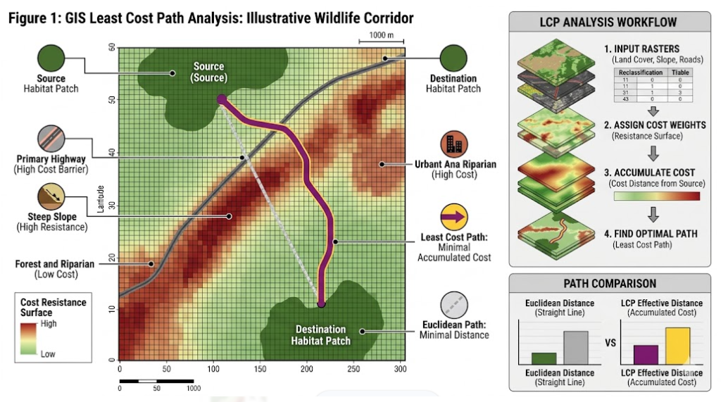
Least cost path analysis identifies the specific route of minimum cumulative cost between two locations through the resistance landscape. Given the accumulated cost surface from a source and a destination point, the least cost path is the line connecting them that minimizes total accumulated resistance.
The calculation is simple once the accumulated cost surface exists.
Starting at the destination cell, the algorithm looks at all neighboring cells and moves to the one with the lowest accumulated cost value. It repeats that step until it reaches the source. The sequence of cells traversed by that back-tracing process is the least cost path.
The path produced is almost never a straight line. It curves through the landscape following the valleys of low resistance in the cost surface, finding the routes where movement is cheapest even when that means traveling a longer absolute distance to avoid a costly barrier.
Wildlife Corridor Identification
Wildlife corridor identification is the most widely recognized application of least cost path analysis in conservation biology.
Habitat fragmentation by roads, agricultural land, and urban development isolates populations of species that require large, connected territories.
When populations cannot disperse between patches, genetic diversity drops, demographic stochasticity increases, and local extinction risk rises.
Identifying corridors through the fragmented matrix is a conservation planning priority, and least cost path analysis is the standard computational method for doing it.
The workflow is direct.
- Define source and destination habitat patches.
- Build a resistance surface reflecting the species’ movement ecology.
- Run cost distance from the source patch.
- Extract the least cost path to the destination.
The resulting line traces the route of minimum cumulative resistance through the matrix: the corridor where habitat connectivity is highest, human disturbance is lowest, and the species has the best chance of moving between patches without mortality or barrier.
Through my work on corridor planning projects, the most useful output is not the single least cost path but a set of corridors derived from multiple cost thresholds.
The lowest-cost path shows the single optimal route. Cost isoclines at 10%, 25%, and 50% above the minimum identify the broader corridor zone where movement cost is low enough to be functionally permeable.
That zone, rather than a single line, is what conservation management can realistically protect and restore.
Infrastructure Route Optimization
Least cost path analysis is equally applicable to infrastructure routing: finding the route for a road, pipeline, power line, or fiber cable that minimizes total construction and environmental impact cost through complex terrain.
The cost raster for infrastructure routing assigns resistance based on factors that drive construction cost and impact:
- steep slopes that require more earthworks,
- protected land that prohibits development,
- watercourses that require crossings,
- settlements that require acquisition and relocation.
The least cost path through that resistance surface finds the route that minimizes total construction difficulty and impact, not just distance.
From my observations on infrastructure planning applications, cost distance analysis is most valuable when competing route options exist and decision-makers need a defensible analytical basis for choosing between them.
The least cost path does not make the decision. It quantifies the tradeoffs between alternatives in a way that is transparent and reproducible.
Real-World Applications of Cost Distance Analysis
Cost distance analysis appears across any application where movement crosses a continuous landscape with spatially variable resistance.

Conservation biology and wildlife corridor planning.
Identifying dispersal routes between fragmented habitat patches is the canonical application. Least cost corridors feed directly into conservation reserve design, land acquisition priorities, and habitat restoration targeting.
Edge effect analysis uses buffer analysis to quantify habitat within defined distances of boundaries; cost distance analysis models whether animals can functionally use that habitat given surrounding resistance.
Off-network health facility accessibility.
In rural areas where significant populations live beyond road network coverage, cost distance analysis extends accessibility modeling into off-road terrain.
A resistance surface combining slope, land cover, and road proximity generates accumulated travel time surfaces that complement network-based service area analysis.
The combination produces a complete picture of accessibility in landscapes where roads exist in some areas and foot travel across terrain is the only option in others.
Hydrological modeling.
Overland flow routing, watershed delineation, and erosion risk modeling all use cost distance logic.
The cost raster for hydrological applications assigns resistance based on the inverse of slope and flow direction, routing water downhill through the path of least gravitational resistance.
Flow accumulation surfaces, which count the number of upstream cells draining through each cell, are built on accumulated cost principles.
Emergency evacuation planning.
Evacuation modeling in post-disaster environments must account for damaged and destroyed infrastructure.
A cost surface that blends road network speed in intact areas with off-road traversability in damaged areas produces evacuation time estimates more realistic than a pure network model in a fragmented infrastructure environment.
How to Run Cost Distance Analysis in GIS
Cost distance analysis requires raster data and a properly built resistance surface. The steps are consistent across platforms.
If you use QGIS:
The GRASS module r.cost runs cost distance analysis natively.
Enable GRASS tools through the Processing Toolbox. You need a cost raster and a source raster (or vector converted to raster) as inputs.
The output is an accumulated cost surface. For least cost path extraction, r.drain traces the minimum cost path from a destination point back to the source through the accumulated cost surface.
Both tools run from the GRASS provider in QGIS’s Processing Toolbox without leaving the QGIS environment.
If you use ArcGIS Pro:
The Spatial Analyst extension provides the Cost Distance (or Distance Accumulation in newer versions) and Cost Path tools.
Cost Distance takes a source raster and cost raster as inputs and produces an accumulated cost surface and a back-direction raster.
Cost Path takes the destination location, the accumulated cost surface, and the back-direction raster and extracts the least cost path.
The full workflow runs from the Spatial Analyst toolbox under Distance.
If you work in Python:
The scikit-image library provides graph-based shortest path tools that work on NumPy arrays. For cost distance analysis, load your cost raster with rasterio, build a pixel graph from it with skimage.graph.MCP_Geometric, and call .find_costs() from your source cell coordinates.
import numpy as np
import rasterio
from skimage.graph import MCP_Geometric

# Load cost raster
with rasterio.open("resistance_surface.tif") as src:
    cost_array = src.read(1).astype(float)
    transform = src.transform

# Define source cell (row, col) from coordinates
source_cell = (50, 30)  # replace with your source coordinates

# Run cost distance
mcp = MCP_Geometric(cost_array)
accumulated_cost, traceback = mcp.find_costs([source_cell])

# Find least cost path to destination cell
destination_cell = (180, 210)  # replace with your destination
path = mcp.traceback(destination_cell)
# path is a list of (row, col) tuples tracing the minimum cost route
Save accumulated_cost back to a GeoTIFF with rasterio using the original transform and CRS for full GIS integration.
If you use R:
The gdistance package is purpose-built for cost distance analysis in R.
Create a TransitionLayer object from your cost raster, correct for geometric distortion with geoCorrection(), then run accCost() for accumulated cost surfaces and shortestPath() for least cost path extraction. The terra package also provides cost distance tools through costDist() in newer versions.
Wrap Up
Cost distance analysis sits in the space between Euclidean distance and network distance: past the point where a straight line works, but in terrain where no discrete infrastructure network exists to route through.
The resistance surface is the heart of the analysis, and building it honestly is the hardest part.
The accumulated cost surface is the engine that turns resistance into a navigable map of travel effort.
The least cost path is the answer: the specific route through the landscape where movement is cheapest, whether that movement is a lynx dispersing between forest patches, a pipeline threading through protected terrain, or a health worker reaching a remote settlement on foot.
What you put into the resistance surface determines what you get out of the least cost path. Get the assumptions right, test them honestly, and report them clearly.
The corridor is only as defensible as the cost raster that produced it.
FAQ
What is cost distance analysis in GIS?
Cost distance analysis measures movement through a landscape of variable resistance, producing an accumulated cost surface where each cell value represents the minimum total travel cost from a source location to that cell through the path of least cumulative resistance. It differs from Euclidean distance, which assumes unconstrained movement, and from network distance, which follows discrete infrastructure. Cost distance is appropriate for any movement process that crosses a continuous landscape where some terrain is easy and some is difficult: wildlife dispersal, overland water flow, off-road accessibility modeling.
What is a cost raster in GIS?
A cost raster is a raster layer where each cell value represents the resistance or friction of moving through that cell. High values indicate high resistance; low values indicate easy passage. Building a cost raster requires assigning resistance values to landscape factors relevant to the movement process being modeled: land cover classes, slope, road proximity, human disturbance, or other variables depending on the application. The cost raster encodes all of the analyst’s assumptions about how the modeled phenomenon responds to the landscape, which makes it both the central analytical component and the most judgment-dependent step in the analysis.
What is least cost path analysis used for in GIS?
Least cost path analysis identifies the specific minimum-cost route between two locations through a resistance landscape, by back-tracing from a destination through the accumulated cost surface to the source. The primary applications are wildlife corridor identification (finding dispersal routes between fragmented habitat patches), infrastructure route optimization (finding the lowest-impact corridor for roads, pipelines, and power lines through complex terrain), and emergency evacuation routing through partially damaged infrastructure. The path produced is almost never a straight line; it curves through the landscape following the valleys of least resistance in the cost surface.
How is cost distance analysis different from buffer analysis?
Buffer analysis creates geometric distance zones around features using straight-line Euclidean distance, assuming movement radiates equally in all directions. Cost distance analysis routes movement through a resistance surface where terrain varies in its traversability, producing accumulated cost zones that follow the contours of least resistance rather than expanding as circles. Buffer analysis is appropriate for regulatory geometric setbacks and preliminary screening. Cost distance analysis is appropriate when the phenomenon being modeled encounters spatially variable terrain resistance: wildlife movement, overland flow, off-road accessibility.
What software runs cost distance analysis?
Cost distance analysis is available in all major GIS platforms. QGIS runs it through the GRASS modules r.cost (accumulated cost surface) and r.drain (least cost path extraction). ArcGIS Pro runs it through the Cost Distance and Cost Path tools in the Spatial Analyst toolbox, or through the newer Distance Accumulation tool. In Python, the skimage.graph.MCP_Geometric class handles cost distance and path extraction on NumPy arrays loaded from raster files. In R, the gdistance package provides accCost() for accumulated cost and shortestPath() for least cost paths.
What’s Next
Cost distance analysis closes the proximity analysis toolkit.
Together, the four articles in this series cover the full family of distance reasoning in GIS: Euclidean distance for unconstrained space, buffer analysis for geometric zone creation, network distance for infrastructure-based mobility, and cost distance for resistance-landscape movement.
For deeper work on the ecological applications covered in this article, the SDM (species distribution modeling) content series covers how cost distance outputs feed into habitat connectivity modeling and species range analysis.
Working on a cost distance project (building a resistance surface, troubleshooting path extraction, or interpreting accumulated cost results)?
Drop your question in the comments.
Happy mapping!