What Is Geospatial Modeling? A Complete Guide to Spatial Models in 2026

A city is planning a new light rail line. Geospatial analysis can tell you where people currently live, how far they are from existing transit stops, and which neighborhoods are underserved right now.

But it can’t tell you what happens ten years after the line opens.

Geospatial modeling can. It can simulate how land use shifts along the corridor, how population density responds to improved accessibility, how travel patterns reorganize across the network — before a single track is laid, before a single dollar is committed.

Analysis describes the present. Modeling tests the future.

What Is Geospatial Modeling?

Geospatial modeling is the process of building computational representations of real-world geographic phenomena to simulate processes, predict outcomes, and test scenarios in spatial context.

It is the most forward-looking layer of the geospatial field. This is the point where data and analysis become simulation and foresight.

Where geospatial analysis describes and measures what exists in the landscape, geospatial modeling generates representations of what could exist under different conditions, at different times, in response to different decisions.

A geospatial model is not a static picture of the world.

It is a dynamic system that responds to inputs, follows spatial rules, and produces outputs that reveal consequences before they become reality.

Think of it as the difference between a photograph and a flight simulator.

A photograph — like a map or an analytical output — captures the state of something at a moment in time with precision and fidelity.

A flight simulator — like a geospatial model — represents how a system behaves, responds to inputs, and evolves under different conditions. Both are valuable. They serve fundamentally different purposes.

Geospatial modeling draws on everything that precedes it in the geospatial stack.

Remote sensing data provides the input layers. GNSS positioning grounds the model in real-world coordinates. GIS technology provides the processing environment. Geospatial analysis provides the pattern recognition and statistical relationships that the model encodes.

Modeling is where the full capacity of the geospatial field converges on a single question: what will happen, where, and under what conditions?

How Is Geospatial Modeling Different From Geospatial Analysis?

This distinction is the most important thing to establish clearly. It’s the question that confuses even experienced GIS professionals.

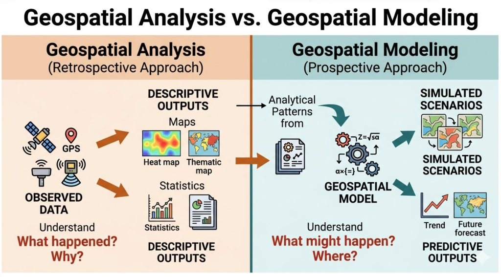
Geospatial analysis is retrospective and descriptive.

It works with existing data to identify patterns, measure relationships, and characterize the current state of spatial phenomena.

It answers questions like:

• where are the flood-prone areas?
• Which neighborhoods lack transit access?
• How has forest cover changed over the past decade?

The output is knowledge about what is. It is grounded in observed data, validated against reality.

Geospatial modeling is prospective and generative.

It uses the patterns and relationships revealed by analysis to simulate processes and project outcomes into hypothetical or future states.

It answers questions like:

• Where will floods occur if rainfall intensity increases by 20 percent?
• How will transit accessibility change if a new station opens?
• How much forest will remain in 2040 if current deforestation rates continue?

The output is knowledge about what could be — dependent on assumptions, sensitive to input quality, and always requiring validation.

The two are deeply connected.

A good geospatial model is always built on a foundation of rigorous geospatial analysis — the patterns encoded in the model come from analyzing observed data.

But the purpose shifts from measurement to simulation, and that shift demands a different set of methods, tools, and critical habits.

As I’ve observed working across analytical and modeling projects, the most common mistake practitioners make is treating model outputs with the same confidence they apply to analytical results.

Analysis describes what the data shows. Modeling describes what the model predicts — and those are different things, with different uncertainty profiles.

What Are the Main Types of Geospatial Models?

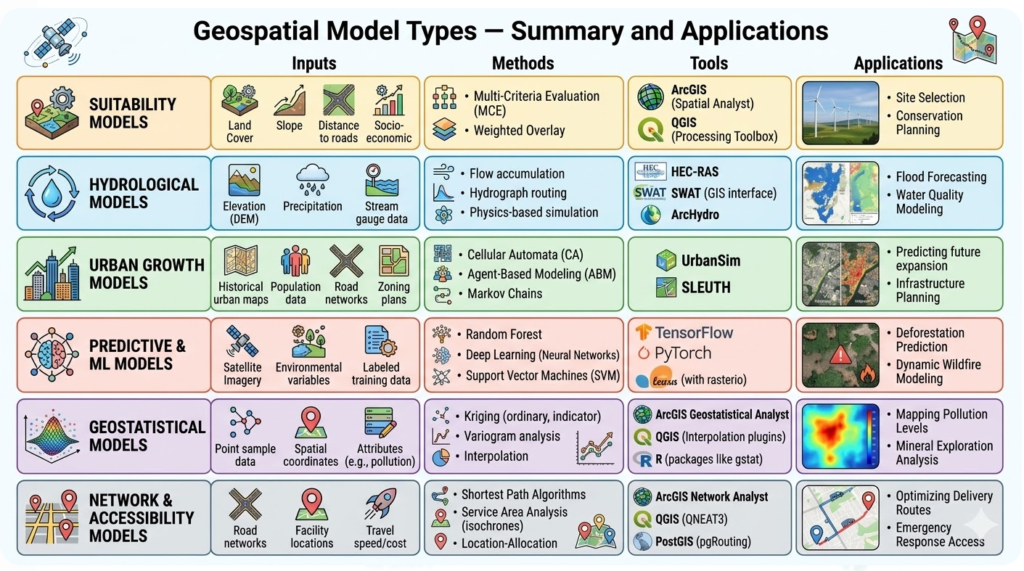
Geospatial modeling encompasses a diverse family of model types, each designed for a different class of spatial problem.

Understanding which type fits which question is a core competency — using the wrong model for a problem produces outputs that look authoritative but answer the wrong question entirely.

Suitability Models

Suitability modeling identifies locations that best meet a defined set of spatial criteria, weighted by their relative importance.

It is the most widely used geospatial modeling approach in land use planning, conservation, and infrastructure siting — and it is typically the first type of geospatial model a GIS practitioner builds.

The structure is straightforward.

You define the criteria that characterize a suitable location for the target use — proximity to roads, slope below a threshold, soil type, distance from sensitive habitats, land ownership.

You assign weights to each criterion reflecting its relative importance. You reclassify each input layer into a common suitability scale. Then you combine them through weighted overlay to produce a continuous suitability surface across the study area.

The output is a map that ranks every location by its overall suitability (from least suitable to most suitable), given the criteria and weights you defined.

Decision-makers can then identify the highest-suitability zones, overlay additional constraints, and explore how the suitability surface changes if weights are adjusted.

Suitability models are used to site solar farms, identify conservation priority areas, select hospital locations, find optimal agricultural expansion zones, and dozens of other placement decisions where multiple spatial criteria must be balanced simultaneously.

Hydrological Models

Hydrological models simulate the movement, accumulation, and behavior of water across terrain and through drainage networks.

They are among the most consequential geospatial models in practice. Their outputs directly inform flood risk management, dam safety assessment, watershed conservation, stormwater infrastructure design, and drought response planning.

The foundation of most hydrological modeling in GIS is the Digital Elevation Model.

From a DEM, the model derives flow direction (which way water moves across each cell), flow accumulation (how much upstream area drains to each cell), stream networks (where accumulated flow exceeds a threshold), and watershed boundaries (the area draining to a specific outlet point).

These derived layers form the spatial framework for simulating what happens to precipitation as it moves through a landscape.

More sophisticated hydrological models like SWAT (Soil and Water Assessment Tool) incorporate soil type, land cover, vegetation, and climate inputs to simulate not just where water flows but how much, how fast, and under what conditions flooding, erosion, or drought occurs.

As I’ve found working with watershed models, the relationship between DEM resolution and model accuracy is one of the most underappreciated factors in hydrological modeling — a coarse DEM produces a coarse stream network, and errors in the stream network propagate through every downstream output.

Urban Growth Models

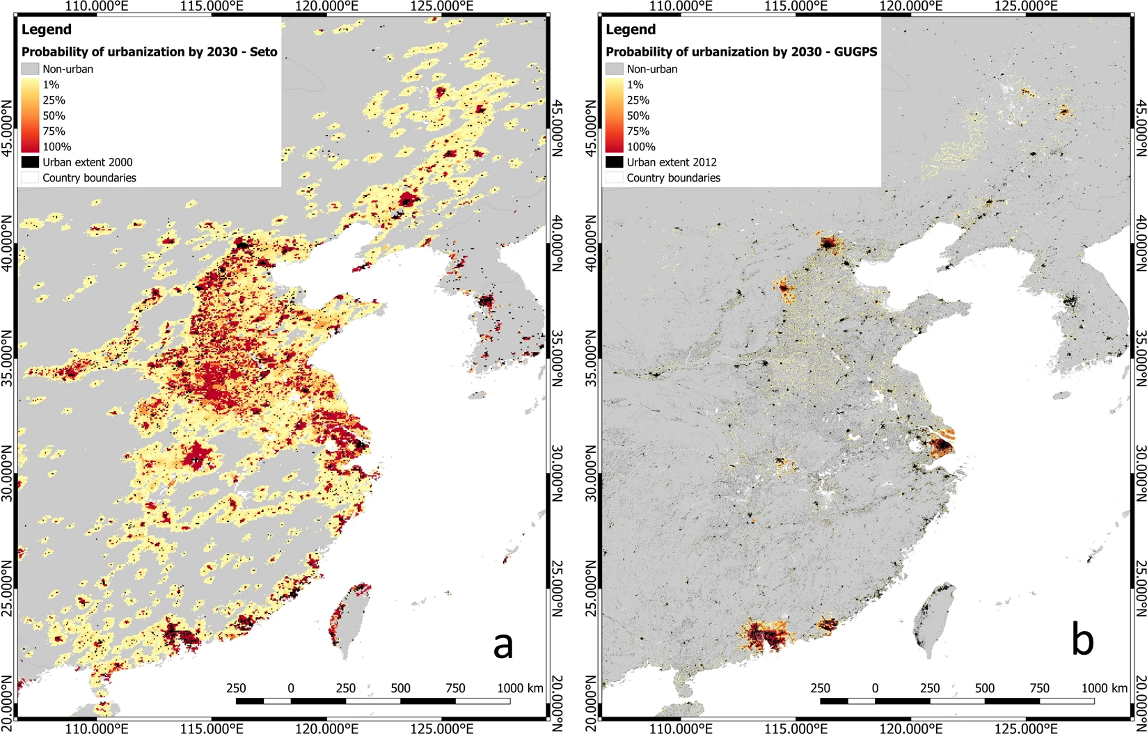
Urban growth models simulate how cities expand, densify, and transform over time in response to population growth, economic development, infrastructure investment, and planning policy. They are the primary tool for long-range urban planning, regional land use policy, and infrastructure investment prioritization.

The most widely used computational approach for urban growth modeling is cellular automata.

CA is a modeling framework where the landscape is represented as a grid of cells, each in one of several possible states (urban, agricultural, forest, water), and where transition rules determine how each cell’s state changes based on the states of its neighbors and a set of driving variables.

SLEUTH — one of the most extensively validated urban growth models — uses historical urban extent data to calibrate transition probabilities and project future growth under different development scenarios.

Agent-based models take a different approach, simulating the decisions of individual actors — households, developers, businesses — and letting urban patterns emerge from the aggregate of those decisions.

These models are more computationally intensive but better suited to questions about how behavioral change or policy interventions would reshape urban form.

Land change simulation platforms like TerrSet’s Land Change Modeler combine historical change analysis with Markov chain modeling to project future land cover transitions across regional extents.

Predictive and Machine Learning Models

Predictive geospatial models use spatial variables such as environmental conditions, demographic characteristics, infrastructure proximity, and historical patterns to predict the probability or magnitude of a phenomenon at locations where no direct measurement exists, or at future time points.

Species distribution models are one of the most mature applications.

They use records of where a species has been observed, combined with environmental raster layers representing climate, vegetation, topography, and soil conditions, to model the probability of suitable habitat across the full landscape — including areas never surveyed.

MaxEnt, one of the most widely used species distribution modeling algorithms, applies a maximum entropy approach to predict species occurrence probability from presence-only data and environmental predictors.

Machine learning has expanded the predictive modeling toolkit substantially.

Random forest classifiers applied to spatial data can model crop yield potential, landslide susceptibility, wildfire risk, and urban flood vulnerability, helps learning complex nonlinear relationships between spatial predictor variables and observed outcomes that traditional statistical models struggle to capture.

The critical challenge in spatial machine learning is spatial autocorrelation, so standard cross-validation techniques that randomly split training and test data violate the independence assumption when observations are spatially clustered.

Spatial cross-validation, which ensures that test observations are geographically separated from training observations, is essential for producing honest accuracy estimates in spatial predictive models.

Geostatistical Models

Geostatistical models build continuous spatial surfaces from discrete point observations, using statistical models of spatial autocorrelation to produce both interpolated values and rigorous estimates of prediction uncertainty.

They are the appropriate modeling approach when the question involves estimating a continuous spatial variable (soil nutrient concentration, groundwater depth, air pollutant concentration, annual rainfall) across a landscape from a finite set of sample points.

Kriging is the foundational geostatistical method. It models the spatial autocorrelation structure of a variable using a semivariogram and uses that structure to produce optimal, unbiased estimates at unmeasured locations.

Ordinary kriging is the standard approach for stationary spatial variables. Universal kriging incorporates a spatial trend component. Indicator kriging estimates the probability that a variable exceeds a threshold rather than estimating its value directly. It is useful for risk mapping applications.

The distinction between geostatistical modeling and simple spatial interpolation is the explicit treatment of uncertainty.

A kriging model doesn’t just produce an estimated surface. It produces a prediction variance surface alongside it, showing where estimates are reliable and where they are uncertain.

That uncertainty surface is as analytically important as the estimated values, and ignoring it leads to overconfident conclusions about spatial patterns in data that is actually quite sparse.

Network and Accessibility Models

Network and accessibility models simulate movement, flow, and access through spatial networks: road systems, transit routes, utility corridors, river networks, and pedestrian paths.

They go beyond the network analysis operations described in the geospatial analysis article to build full simulation environments where demand, capacity, congestion, and behavioral response interact dynamically.

Transport models are one of the most sophisticated applications.

A regional transport model simulates how the full population of travelers distributes across a transport network under current conditions and how that distribution shifts in response to new infrastructure, changed travel costs, or altered land use patterns.

These models are the standard tool for evaluating major transport infrastructure investments and inform decisions worth billions of dollars in capital expenditure.

Evacuation modeling simulates how a population moves through a road network during an emergency, identifying bottlenecks, estimating clearance times, and optimizing shelter placement and route guidance.

Supply chain network models optimize the flow of goods through distribution networks, minimizing cost while respecting capacity and demand constraints.

Accessibility models calculate how reachable essential services (hospitals, schools, food retailers, employment centers) are for different population groups, supporting equity-focused planning and resource allocation.

What Tools Are Used for Geospatial Modeling?

The geospatial modeling tool landscape is broader and more specialized than the analysis tool landscape. Choosing the right tool depends on model type, data volume, required precision, and the technical environment of your organization.

Desktop GIS — QGIS and ArcGIS Pro

Both QGIS and ArcGIS Pro provide graphical model building environments that let analysts chain geospatial operations into automated, repeatable workflows without writing code.

QGIS’s Graphical Modeler and ArcGIS Pro’s ModelBuilder both support building multi-step models visually. They are connecting input datasets, processing operations, and output products in a flowchart-style interface.

ArcGIS Pro’s Spatial Analyst extension provides a comprehensive raster modeling toolkit — surface analysis, hydrological modeling, suitability analysis, and interpolation — that covers most of the core geospatial modeling methods.

QGIS accesses much of the same functionality through its Processing Toolbox, which integrates tools from GRASS GIS, SAGA, and GDAL alongside QGIS’s own algorithms.

For practitioners building moderately complex models in an interactive environment, desktop GIS platforms provide the most accessible entry point into geospatial modeling.

Specialized Modeling Software

Some geospatial modeling domains have dedicated software tools built specifically for their problem domain that go far deeper than general-purpose GIS platforms in their modeling capability.

SWAT (Soil and Water Assessment Tool) is the standard platform for watershed-scale hydrological modeling, simulating water balance, sediment transport, and nutrient cycling across complex drainage systems.

TerrSet’s Land Change Modeler provides a complete environment for land cover change analysis, transition potential modeling, and future land use scenario simulation.

NetLogo is the most widely used platform for agent-based spatial modeling, supporting the simulation of individual actor behavior and emergent spatial patterns.

For practitioners working in these specialized domains, learning the dedicated tool alongside a general GIS platform produces substantially better modeling outcomes than trying to replicate domain-specific functionality in a general-purpose environment.

Programming — Python and R

Python and R provide the most flexible, reproducible, and extensible environments for geospatial modeling, particularly for predictive and machine learning models that require custom workflows and rigorous validation frameworks.

Python’s scikit-learn library provides a comprehensive machine learning toolkit that integrates cleanly with GeoPandas spatial data structures. The PySAL library provides spatial econometric and geostatistical modeling tools including spatial weights matrices, spatial regression models, and exploratory spatial data analysis methods.

For deep learning applications PyTorch and TensorFlow both support geospatial modeling workflows when combined with rasterio and spatial data preprocessing pipelines.

R’s modeling ecosystem is particularly strong for geostatistical and statistical spatial modeling.

The gstat package implements the full range of kriging methods with variogram modeling. The randomForest and caret packages support spatial predictive modeling, and the blockCV package implements spatial cross-validation — the correct validation approach for spatially autocorrelated data.

From my professional practice, R remains the strongest environment for rigorous geostatistical modeling and spatial statistics, while Python leads for machine learning integration and large-scale data pipeline development.

Cloud Platforms — Google Earth Engine and ArcGIS Online

Google Earth Engine supports large-scale raster-based modeling workflows at continental and global extents that desktop platforms cannot practically handle.

Its JavaScript and Python APIs provide full programmatic control over modeling workflows, and its built-in machine learning tools including Random Forest and SVM classifiers make predictive spatial modeling accessible without local infrastructure.

ArcGIS Online’s Raster Analysis tools and Living Atlas datasets support web-based scenario modeling and suitability analysis for organizations that need collaborative, browser-accessible modeling environments.

For teams that need to share model inputs, outputs, and scenarios across multiple stakeholders without requiring desktop GIS installation, cloud platforms provide the most practical delivery environment.

What Does a Geospatial Modeling Workflow Look Like?

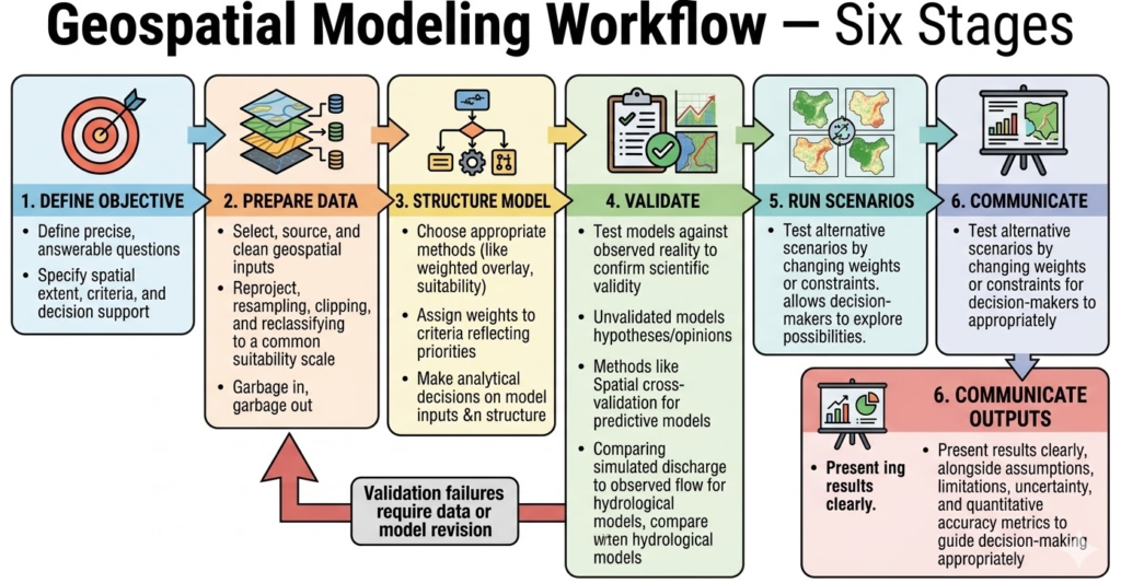
Geospatial modeling follows a structured workflow that differs from analytical workflows in one critical respect: validation is not optional.

A model that has not been tested against observed reality is not a scientific output, only a hypothesis.

Here is what a complete modeling workflow looks like, using a land suitability model for solar farm site selection as the example.

Stage 1: Define the Modeling Objective

Every geospatial model begins with a precise, answerable question.

For the solar suitability model: which locations in this region are most suitable for utility-scale solar farm development, given solar irradiance, land cover, slope, grid proximity, and environmental sensitivity constraints?

A well-defined modeling objective specifies the spatial extent, the criteria and their relative importance, the output format required, and the decision the model will support. Ambiguous objectives produce models that answer the wrong question with impressive precision.

A failure mode more dangerous than a model that produces obviously wrong results.

Stage 2: Select and Prepare Input Data

For example, the solar suitability model requires five input layers:

• a solar irradiance surface (from NASA or PVGIS),
• a land cover classification (from Sentinel-2 or a national dataset),
• a slope layer derived from a DEM,
• a distance-to-grid layer calculated from transmission infrastructure data, and
• an environmental sensitivity layer combining protected areas, wetlands, and biodiversity hotspots.

Each layer needs to be reprojected to a common coordinate reference system, resampled to a consistent spatial resolution, clipped to the study area boundary, and reclassified to a common suitability scale (typically 1 to 5 or 1 to 9).

The quality of this preparation stage determines the reliability of every output the model produces.

Garbage in, garbage out is a cliché because it is true. And in geospatial modeling, the garbage is often invisible until the validation stage exposes it.

Stage 3: Choose and Structure the Model

For land suitability, weighted overlay is the appropriate model structure.

Assign weights to each criterion reflecting stakeholder priorities :

• solar irradiance might carry 40 percent of the total weight,
• slope 20 percent, grid proximity 20 percent,
• land cover 15 percent,
• and environmental sensitivity as a hard constraint that excludes certain areas entirely regardless of other scores.

Model structure choices, which criteria to include, how to weight them, whether to use hard constraints or soft scores, are analytical decisions that require domain knowledge, stakeholder input, and explicit documentation.

As I’ve found in suitability modeling projects, the weighting decisions are almost always more contested than the technical implementation. Making them transparent and adjustable is as important as getting them right.

Stage 4: Calibrate and Validate the Model

For predictive models, calibration means fitting model parameters to observed data.

For suitability models, validation means testing whether high-suitability zones correspond to locations that expert knowledge or observed outcomes would identify as genuinely suitable.

Validation approaches vary by model type.

Predictive models use spatial cross-validation — training on one geographic subset, testing on a spatially separated subset — to produce honest accuracy estimates.

Hydrological models are validated by comparing simulated streamflow at gauge stations against observed discharge records.

Urban growth models are calibrated using historical urban extent data from one period and validated by comparing model projections with observed growth in a subsequent period.

An unvalidated model is an opinion dressed as analysis.

In my professional opinion, no geospatial model output should inform a consequential decision without a documented validation procedure, regardless of how sophisticated the modeling approach or how credible the input data.

Stage 5: Run Scenarios

The power of a validated model is its ability to test scenarios.

For the solar suitability model:

• How does the suitability surface change if grid connection distance is given more weight?
• What happens to available suitable area if slope constraints are tightened?
• How do results differ under high versus low environmental sensitivity constraints?

Scenario analysis is where geospatial modeling delivers its most distinctive value as they explore a space of possibilities before committing to a decision.

Each scenario run is computationally fast once the model is built and validated. The insights from comparing scenarios often reshape the decision framing entirely.

Stage 6: Communicate Outputs

Model outputs need to communicate not just the results but the assumptions, limitations, and uncertainty embedded in them.

A suitability map without a description of the criteria weights, data sources, and validation approach is incomplete and potentially misleading if decision-makers treat it as more certain than it is.

Effective model communication includes the primary output map, a sensitivity analysis showing how results change under different parameter assumptions, a clear statement of the model’s limitations. For predictive models, quantitative accuracy metrics that allow decision-makers to calibrate their confidence appropriately.

What Are the Limitations of Geospatial Modeling?

Geospatial models are powerful tools.

They are also simplifications of reality, and understanding their limitations is as important as understanding their capabilities.

From what I’ve seen across many modeling projects, the analysts who produce the most trustworthy model outputs are consistently the ones who are most honest about what their models cannot do.

All models are simplifications by design.

A geospatial model encodes a set of rules about how a spatial system behaves. Those rules are necessarily incomplete — they omit variables that are difficult to measure, assume relationships that hold on average but not everywhere, and represent continuous processes as discrete steps. The art of geospatial modeling is knowing which simplifications are acceptable for the question at hand and which ones would invalidate the output.

Output quality is bounded by input data quality.

A hydrological model built on a coarse, outdated DEM produces a coarse, unreliable stream network. A species distribution model trained on occurrence records with significant geographic bias produces a biased habitat map. The model cannot compensate for poor input data — it amplifies the errors and presents them with the authority of a computational output.

Validating future and hypothetical scenarios is inherently difficult.

A model projecting urban growth to 2050 cannot be validated against 2050 observations, as those don’t exist yet.

Proxy validation approaches exist, but they all involve assumptions that future conditions will resemble past conditions in ways that may not hold. Future-facing model outputs should always be presented as scenarios, not predictions.

Scale and resolution choices significantly affect results.

A flood model run at 10-meter DEM resolution produces different inundation extents than the same model run at 30-meter resolution — sometimes dramatically so.

A species distribution model trained on 1-kilometer climate grids cannot reliably predict habitat at 100-meter resolution.

Matching model resolution to the scale of the decision it informs is a fundamental modeling design choice that is frequently underemphasized.

Where Is Geospatial Modeling Applied?

Geospatial modeling supports decision-making wherever the consequences of spatial choices extend into the future or involve systems too complex to characterize through analysis alone.

Environmental and Climate Modeling

Environmental agencies and research institutions use geospatial models to project climate change impacts on land cover, water availability, species distributions, and coastal flooding.

Climate downscaling models translate coarse global climate projections into regional-scale spatial outputs that local planners and resource managers can use.

Ecosystem service models quantify the spatial distribution of services like carbon sequestration, water purification, and pollination under current and projected future land cover scenarios.

Urban Planning and Transport

Urban growth models inform long-range regional planning by projecting where development pressure will be greatest under different infrastructure and policy scenarios.

Transport models evaluate the ridership, congestion, and accessibility impacts of proposed transit investments before construction begins.

Land use transport interaction models simulate the feedback between urban form and travel behavior over multi-decade planning horizons — the standard tool for metropolitan strategic planning worldwide.

Disaster Risk and Resilience

Flood simulation models delineate inundation extents under design storm events — the spatial outputs that define flood zone boundaries in insurance, planning, and building regulations.

Landslide susceptibility models identify unstable slopes that represent risk to infrastructure and communities.

Earthquake loss estimation models project the spatial distribution of structural damage and casualties from scenario seismic events.

Evacuation models simulate population movement under emergency conditions, optimizing shelter locations and route guidance.

Agriculture and Food Security

Crop yield potential models combine soil, climate, and topographic inputs to project where agricultural productivity is highest, and how it will shift under climate change scenarios.

Irrigation demand models simulate water requirements across agricultural landscapes under different crop mix and climate assumptions.

Food security scenario models project the spatial distribution of production capacity and vulnerability under combined climate, economic, and demographic change.

Public Health

Spatial disease transmission models project how infectious diseases spread through populations that are distributed across geographic space, enabling public health agencies to target interventions where they will have the greatest impact.

Health impact assessment models project how changes in air quality, urban heat, or greenspace access would affect population health outcomes across a city or region.

Facility location models optimize the placement of health infrastructure to maximize accessibility for underserved populations.

Conservation and Biodiversity

Species distribution models project suitable habitat for target species across unsampled landscapes and under future climate scenarios — the primary tool for conservation planning under climate change.

Connectivity models identify and prioritize wildlife corridors that maintain movement between habitat patches in fragmented landscapes.

Systematic conservation planning models — implemented in tools like Marxan — identify the minimum set of areas that would meet biodiversity representation targets at minimum cost, given competing land use pressures.

How Do You Build Your First Geospatial Model?

Geospatial modeling rewards practice more than almost any other component of the field. The concepts become clear when you build a model, adjust its parameters, and see how the output responds. Here are three entry points matched to different skill levels.

Beginner: Weighted overlay suitability model in QGIS

Download QGIS and source three to four raster layers for your area of interest — a DEM for slope, a land cover layer from Copernicus or USGS, and a distance-to-roads layer you can generate from an OpenStreetMap road network.

Reclassify each layer to a common 1-to-5 suitability scale using the Reclassify by Table tool.

Combine them using the Raster Calculator with your chosen weights. The result is your first suitability surface.

Adjust the weights and observe how the output changes — that sensitivity exploration is one of the most valuable learning experiences in geospatial modeling.

Intermediate: Hydrological watershed model from a DEM

Download a DEM for a watershed area of interest from USGS or Copernicus.

In QGIS, use the SAGA provider through the Processing Toolbox to run the full hydrological modeling chain: fill sinks, calculate flow direction, calculate flow accumulation, extract stream networks at a threshold, and delineate watershed boundaries for a set of outlet points.

Compare your modeled stream network against actual river locations from OpenStreetMap. The agreement — and disagreement — between modeled and observed streams is your first practical lesson in hydrological model validation.

Advanced: Species distribution model in R with spatial cross-validation

Download species occurrence records from GBIF for a target species and environmental raster layers from WorldClim or CHELSA.

Fit a Random Forest species distribution model using the caret package. Then implement spatial cross-validation using the blockCV package — partitioning your occurrence data into spatially separated blocks rather than random folds.

Compare the accuracy metrics from random cross-validation versus spatial cross-validation.

The difference will almost certainly be larger than you expect, and it will permanently change how you think about model validation in spatially autocorrelated data.

Wrap Up

Geospatial modeling is the most forward-looking layer of the geospatial field.

It takes the data that remote sensing collects, the positioning that GNSS provides, the infrastructure that GIS technology builds, and the patterns that geospatial analysis reveals — and uses all of it to simulate, predict, and test.

It is where the geospatial field moves from describing the world to shaping decisions about its future.

The six model types — suitability, hydrological, urban growth, predictive and machine learning, geostatistical, and network and accessibility — cover the modeling vocabulary you need to work across the full range of spatial decision problems.

The tools are largely accessible. The workflows are learnable. And the field rewards rigor above everything else.

Build models that are honest about their assumptions. Validate before you communicate. Present uncertainty alongside results. And never confuse a model’s output with reality — only with a better-informed approximation of it.

Build the model. Test it. Then trust the process.

FAQ

What is geospatial modeling in simple terms?

Geospatial modeling is the process of building computational representations of geographic phenomena to simulate how they behave, predict where they will occur, or test what would happen under different conditions. Where geospatial analysis describes what currently exists in the landscape, geospatial modeling projects what could exist — under different inputs, at future times, or in response to different decisions. It is the tool that turns spatial data and analytical patterns into foresight.

What is the difference between geospatial modeling and geospatial analysis?

Geospatial analysis is retrospective and descriptive — it works with existing data to identify patterns, measure relationships, and characterize current spatial phenomena. Geospatial modeling is prospective and generative — it uses those patterns and relationships to simulate processes and project outcomes into hypothetical or future states. Analysis answers what is here and how it relates. Modeling answers what will happen here if conditions change. The two are deeply connected — models are built on analytical foundations — but they serve different purposes and require different critical habits.

What are the main types of geospatial models?

The six core geospatial model types are suitability models (identifying optimal locations based on weighted spatial criteria), hydrological models (simulating water flow and drainage across terrain), urban growth models (simulating how cities expand and transform over time), predictive and machine learning models (projecting phenomena at unmeasured locations or future times), geostatistical models (building continuous surfaces from point observations with uncertainty estimation), and network and accessibility models (simulating movement and access through spatial networks).

What tools are used for geospatial modeling?

Geospatial modeling tools span four categories. Desktop GIS platforms — QGIS Graphical Modeler and ArcGIS ModelBuilder with Spatial Analyst — support interactive model building for most standard model types. Specialized software — SWAT for hydrology, TerrSet for land change, NetLogo for agent-based models — provides domain-specific depth. Programming environments — Python with scikit-learn, PySAL, and PyTorch, and R with gstat, randomForest, and blockCV — support reproducible and custom modeling workflows. Cloud platforms — Google Earth Engine and ArcGIS Online — enable large-scale and collaborative modeling.

What is a suitability model in GIS?

A suitability model identifies locations that best meet a defined set of spatial criteria, weighted by their relative importance. It works by reclassifying multiple input raster layers to a common suitability scale, assigning weights to each layer, and combining them through weighted overlay to produce a continuous suitability surface. The output ranks every location in the study area by its overall suitability for the target use. Suitability models are used for site selection, conservation prioritization, infrastructure planning, and land use decision-making.

How do I get started with geospatial modeling?

The most accessible starting point is a weighted overlay suitability model in QGIS — it requires only free software, freely available raster data, and the Raster Calculator tool. Download a DEM, a land cover layer, and a roads layer for your area of interest, reclassify each to a common suitability scale, combine them with chosen weights, and explore how the output changes as you adjust those weights. For practitioners with Python experience, fitting a Random Forest species distribution model with spatial cross-validation in R or Python is the most instructive introduction to spatial predictive modeling.

You’ve Reached the End of the Geospatial Fundamentals Series

This article is the final piece in the Better Mapmaker geospatial fundamentals cluster. Together, the four articles cover the full conceptual foundation of the field:

The what is geospatial article establishes what the field means and why location matters.

The what is geospatial technology article maps the full tool stack from sensors to web platforms.

The geospatial data article covers what spatial data is and how they are differ with other types of data.

The geospatial analysis article covers the seven core analytical methods and how they work.

And this article completes the picture with the modeling layer — where analysis becomes simulation and foresight.

Drop a comment below and tell us where you are and where you’re headed. Let’s figure out the next step together.

Happy mapping!