What Are Thiessen Polygons in GIS? Understand the Voronoi Diagram

Learn what Thiessen polygons are in GIS, how they are constructed, their applications in hydrology and service planning, and their core limitations.

In 1911, meteorologist Alfred Thiessen needed a way to estimate rainfall across a watershed using only point measurements from scattered rain gauges.

His solution was geometric: draw boundaries equidistant between each pair of adjacent gauges, partition the watershed into zones, and weight each gauge’s measurement by the area of its zone.

The method worked well enough that it became standard hydrological practice and carried his name for the next century.

Georgy Voronoi, a Ukrainian mathematician, had described the same geometric construction a decade earlier from a pure mathematics perspective.

Neither man knew the other’s work. The result was the same structure with two names that GIS practitioners still use interchangeably today.

That origin story tells you something useful about Thiessen polygons: they were invented to solve a specific, bounded problem.

Understanding what that problem is determines when the tool fits and when it does not.

What Are Thiessen Polygons in GIS?

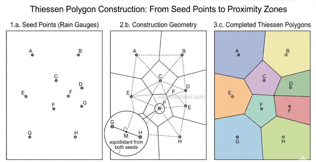
Thiessen polygons are a spatial partitioning method that divides an area into zones based on proximity to a set of input points.

Every location within a Thiessen polygon is closer to that polygon’s seed point than to any other seed point in the dataset.

In GIS, Voronoi diagram analysis and Thiessen polygon construction refer to the same operation. Mathematicians also call the structure a Dirichlet tessellation, though that term rarely appears in GIS software interfaces.

Think of it as a territorial claim: each seed point claims the surrounding space out to the midpoint between itself and its neighbors.

The boundary between two adjacent polygons is not drawn arbitrarily. It falls precisely at the locus of points equidistant from the two seeds, a perpendicular bisector of the line connecting them. Where three polygon territories meet, all three boundaries intersect at a point equidistant from three seeds simultaneously.

The result is a set of polygons that tiles the entire analysis extent with no gaps and no overlaps.

Every location in the study area belongs to exactly one polygon, assigned to exactly one seed point: the nearest one.

The Geometry of Voronoi Construction

The construction algorithm works from a set of input seed points and produces polygon boundaries by finding, for every pair of neighboring seeds, the perpendicular bisector of the line segment connecting them. Those bisectors become the polygon edges.

Each resulting polygon is a convex shape.

No Thiessen polygon has an interior angle greater than 180 degrees, which is a direct consequence of the equidistant boundary rule.

The size and shape of each polygon reflect the spacing and arrangement of the surrounding seeds: seeds in a dense cluster produce small, compact polygons; an isolated seed far from its neighbors claims a large territory extending well beyond where a denser arrangement would have drawn the boundary.

The Delaunay triangulation is the geometric dual of the Voronoi diagram.

Connect the seed points whose polygons share a boundary, and you produce a triangulation of the seed points with a specific property: the circumcircle of each triangle contains no seed point other than its own three vertices.

GIS platforms that compute Voronoi diagrams often compute the Delaunay triangulation simultaneously, since both structures derive from the same underlying proximity geometry.

What Are Thiessen Polygons Used For?

Thiessen polygons answer one specific spatial question: given a set of point locations, which is nearest to every other location in the study area?

That question recurs across domains, which explains why the same geometric construction appears in hydrology, service planning, ecology, and computational geometry.

Rainfall Estimation in Hydrology

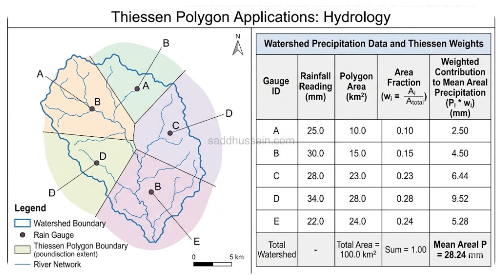
Thiessen polygon hydrology is where the method originated and where it still performs best.

A watershed with rain gauges at several locations has point measurements of precipitation but needs an estimate of total areal rainfall across the entire basin. Simple averaging of gauge readings ignores the fact that some gauges represent larger portions of the watershed than others.

The Thiessen method addresses this directly.

Each gauge’s Thiessen polygon defines the portion of the watershed that gauge represents. Multiply each gauge reading by its polygon’s fraction of the total watershed area, sum the results, and the weighted average gives the mean areal precipitation estimate for the basin.

A gauge surrounded by a 40-square-kilometer polygon contributes proportionally more to the basin estimate than a gauge in a 10-square-kilometer polygon.

The method assumes that precipitation at any point equals the measurement at its nearest gauge.

That assumption holds reasonably well in flat terrain with a dense gauge network. It becomes less defensible in mountainous terrain, where orographic effects cause precipitation to vary sharply over short distances that may not align with Thiessen boundaries.

Service Area Delineation and Facility Planning

Thiessen polygon service area delineation answers a direct planning question: if every resident uses the nearest facility, what catchment does each facility serve?

Applied to hospitals, schools, fire stations, or retail locations, the result is a spatial allocation of the surrounding population to each facility based on geometric proximity.

As I’ve found when reviewing facility planning documents, Thiessen-based catchment zones appear frequently in preliminary planning analyses because they are fast to produce and require no network data.

A hospital planning team can generate Thiessen polygons from a list of facility coordinates in minutes and immediately see which facilities serve large versus small geographic zones.

That speed is the tool’s practical value at the scoping stage. The problem comes when the Thiessen catchment is treated as the final answer rather than a first approximation. The next section covers that limitation in detail.

Ecology and Individual Territory Mapping

In plant ecology and animal behavior research, Voronoi diagrams map the spatial extent of individual organisms’ territories or competitive zones.

Place seed points at individual tree locations and the Voronoi cells approximate the growing space each tree competes for: the area closer to that tree than to any other. The cell area correlates with the tree’s competitive advantage and resource access.

For animal territory analysis, the approach is less biologically precise but still analytically useful.

Voronoi cells around individual animal locations or activity centers give a geometric approximation of exclusive territory extent, which feeds into density estimation and home range analysis.

Computational Geometry and Spatial Databases

Beyond direct GIS applications, Voronoi structures underpin nearest-neighbor search algorithms in spatial databases and geographic information systems themselves.

When a spatial query asks for the nearest point to a query location, a Voronoi-based index locates the answer without exhaustive pairwise distance computation.

Spatial databases and tree-based spatial indices derive their efficiency from the same geometric partitioning that Thiessen used for rain gauges in 1911.

What Is the Core Limitation of Thiessen Polygons?

The Thiessen polygon limitations discussed most often in GIS practice come down to one root cause: the boundaries are equidistant in Euclidean space.

They reflect which seed point is nearest as the crow flies, not which seed point is nearest through the road network, through the pedestrian path network, or through any other real-world movement system.

That distinction does not matter in the original hydrological application.

Rain falls vertically. It does not commute to work or walk to a hospital. The straight-line distance assumption is geometrically correct for precipitation, which is why the Thiessen method has held up for over a century in that domain.

It matters considerably in service planning.

The Road Network Problem

A Thiessen boundary between two hospitals runs through whatever geographic line is equidistant from both facilities in straight-line distance.

That boundary may run through a neighborhood where residents can reach Hospital A in 8 minutes by road and Hospital B in 22 minutes, but where the Euclidean distances to both facilities are nearly equal. The Thiessen polygon assigns those residents to Hospital B’s catchment. The road network would send every one of them to Hospital A.

The error is not random noise. It is systematic.

Thiessen boundaries consistently misallocate populations in areas where physical barriers, sparse road coverage, or asymmetric street networks create large gaps between Euclidean and network distance.

From my perspective, the most consequential misallocations happen in three situations:

• neighborhoods cut off from a nearby facility by a river or rail line with few crossings,
• areas where a major road on one side of a Thiessen boundary creates fast network access to one facility despite greater Euclidean distance, and
• low-density peri-urban areas where the road network is sparse and indirect routes dominate.

When Thiessen Polygons Are Still Appropriate

The limitation is domain-specific, not universal.

Thiessen polygons remain the correct tool in any application where straight-line distance is the genuinely appropriate distance concept.

A common question is Thiessen polygon vs buffer: both are proximity tools, but they answer different questions. A buffer creates a fixed-distance zone around a feature. A Thiessen polygon assigns every location to its nearest feature. Neither is universally superior. The right choice depends on the question.

Hydrological rainfall estimation belongs in this category, as covered above.

Preliminary spatial scoping, where a rough allocation of areas to nearest points is needed before more rigorous analysis, is another legitimate use.

Computational nearest-neighbor indexing uses Voronoi geometry for efficiency, not for behavioral modeling.

In all of these cases, the Euclidean assumption is either appropriate to the phenomenon or explicitly acknowledged as a simplification.

The tool fails specifically when applied to questions about human behavior and mobility: which facility will people actually use, who is actually accessible to a service, which catchment population does a facility realistically serve.

Those questions require network distance.

What Is Network Voronoi Analysis in GIS?

Network Voronoi analysis is the network distance equivalent of Thiessen polygon construction.

Instead of assigning every location to its nearest seed point by straight-line distance, it assigns every location to its nearest seed point by travel time or distance through the road or pedestrian network.

The output polygon boundaries are no longer perpendicular bisectors in Euclidean space. They fall at the points where travel time to two adjacent facilities is equal through the network: the true equidistant boundary given how people actually move.

In areas with symmetric road networks, network Voronoi boundaries approximate Thiessen boundaries. In areas with physical barriers, sparse coverage, or asymmetric street layouts, they diverge substantially.

Network Voronoi analysis requires a topologically correct network dataset with encoded travel impedances, which is more demanding than Thiessen construction.

But for any facility planning application where network accessibility determines which facility people realistically use, it is the correct tool.

GIS platforms handle this differently.

ArcGIS Pro runs network-based service area analysis through the Network Analyst extension, and the intersection of adjacent service area polygons defines the network Voronoi boundary.

QGIS achieves the same result through QNEAT3 or GRASS network tools. The computational demand is higher than Thiessen construction, but the result reflects how the population actually accesses services.

How to Create Thiessen Polygons in GIS

Thiessen polygon construction is straightforward in all major GIS platforms. The input is a point feature layer. The output is a polygon layer.

If you use QGIS:

Thiessen polygon analysis in QGIS runs from Vector > Geometry Tools > Voronoi Polygons. The tool takes your input point layer and an optional buffer percentage that extends the polygons slightly beyond the input extent to avoid clipping near the edges. The output is a polygon layer with one polygon per input point, containing the input point’s attributes joined to the polygon. To clip the result to a study area boundary such as a watershed or administrative region, run a subsequent Vector > Geoprocessing > Intersection or Clip operation.

If you use ArcGIS Pro:

Thiessen polygon analysis in ArcGIS Pro uses the Create Thiessen Polygons tool in the Analysis toolbox under Proximity. Input a feature class of points and specify the output fields you want carried from the input to the polygon layer. ArcGIS Pro also lets you set an extent environment to clip the polygons to a defined boundary automatically. For large point datasets, the tool runs efficiently without additional configuration.

If you work in Python:

Thiessen polygon analysis in Python uses the scipy.spatial.Voronoi function, which computes the Voronoi diagram from a NumPy array of point coordinates. Pair it with shapely and geopandas to convert the output into a GeoDataFrame of polygon geometries that can be written to a GeoPackage or Shapefile.

import numpy as np
import geopandas as gpd
from scipy.spatial import Voronoi
from shapely.ops import voronoi_diagram
from shapely.geometry import MultiPoint, box

# Load your seed points
seeds = gpd.read_file("rain_gauges.gpkg")
seeds = seeds.to_crs(epsg=32637)  # project to metric CRS first

# Build Voronoi diagram clipped to study area extent
boundary = box(*seeds.total_bounds)
multipoint = MultiPoint(list(seeds.geometry))
regions = voronoi_diagram(multipoint, envelope=boundary)

# Convert to GeoDataFrame
voronoi_gdf = gpd.GeoDataFrame(
    geometry=list(regions.geoms),
    crs=seeds.crs
)

# Spatial join to attach seed point attributes
result = gpd.sjoin(voronoi_gdf, seeds, how="left", predicate="contains")
result.to_file("thiessen_polygons.gpkg", driver="GPKG")

The voronoi_diagram function from shapely.ops handles the clipping boundary directly, avoiding the unbounded polygon issue that raw scipy.spatial.Voronoi produces for points near the hull of the input.

If you use R:

The spatstat package computes Voronoi tessellations through dirichlet(). The deldir package is an alternative that produces both the Voronoi diagram and the Delaunay triangulation simultaneously. Both packages return spatial objects compatible with the sf package for further GIS operations.

Wrap Up

Thiessen polygons are a clean solution to a clean problem: partition a continuous space so that every location belongs to its nearest point.

In hydrology, that problem maps precisely onto rainfall estimation from point gauges, and the Thiessen method has earned its century of use. In ecology, it gives a reasonable geometric approximation of competitive territory. In computational geometry, it drives spatial indexing that makes nearest-neighbor queries fast.

In service planning, the problem the method solves is not quite the problem planners need to answer.

Nearest by straight line is not the same as nearest by road. When the difference matters, use network Voronoi analysis. When it does not, Thiessen polygons remain as useful as they were in 1911.

Know which question you are asking. The geometry will follow.

FAQ

What are Thiessen polygons in GIS?

Thiessen polygons are a spatial partitioning method that divides a study area into zones based on proximity to a set of input point features. Every location within a Thiessen polygon is closer to that polygon’s seed point than to any other seed point, with boundaries falling exactly at the line equidistant between adjacent seeds. They are also called Voronoi diagrams, named for mathematician Georgy Voronoi who described the same geometric construction independently from meteorologist Alfred Thiessen. In GIS, the two terms are used interchangeably.

What is the difference between Thiessen polygons and Voronoi diagrams?

Thiessen polygons and Voronoi diagrams are the same geometric structure. The name Thiessen comes from meteorologist Alfred Thiessen, who developed the construction for hydrological rainfall estimation in 1911. The name Voronoi comes from mathematician Georgy Voronoi, who described the same geometry mathematically around a decade earlier. GIS software uses both terms depending on the platform and application domain: ArcGIS Pro uses “Create Thiessen Polygons”; QGIS uses “Voronoi Polygons.” The output is identical.

What are Thiessen polygons used for in GIS?

The primary applications are hydrological rainfall estimation (weighting point gauge measurements by the area each gauge represents in a watershed), service area delineation (preliminary catchment zones around facilities like hospitals, schools, and fire stations), ecological territory mapping (approximating competitive growing space or animal territory extent from point locations), and spatial database indexing (powering nearest-neighbor search algorithms). Hydrology is the application where the straight-line distance assumption is most defensible. Service planning is the application where it is most often misapplied.

What is the main limitation of Thiessen polygons?

Thiessen polygon boundaries reflect Euclidean equidistance, not network equidistance. The boundary between two adjacent facility catchments falls at the point of equal straight-line distance from both facilities, not at the point of equal travel time through the road network. In areas with physical barriers, sparse road coverage, or asymmetric street layouts, these two boundaries diverge significantly. Populations near a Thiessen boundary may be assigned to the geometrically nearest facility even though the road network routes them to a different one. For service planning applications where network accessibility determines facility use, network Voronoi analysis is the correct alternative.

How do Thiessen polygons differ from buffers in GIS?

Buffer analysis creates distance zones around features: rings, corridors, or expanded polygons at a defined distance from each feature. The zones can overlap and do not necessarily cover the full study area. Thiessen polygons partition the study area exhaustively: every location belongs to exactly one polygon, with no gaps and no overlaps. A buffer answers the question “what falls within distance X of this feature?” A Thiessen polygon answers the question “which feature is nearest to this location?” They are complementary tools that address different spatial questions.

Can you run Thiessen polygon analysis in QGIS, ArcGIS Pro, and Python?

Yes, all three platforms support Thiessen polygon construction. QGIS runs it through Vector > Geometry Tools > Voronoi Polygons, with an optional buffer percentage parameter and a subsequent clip step to limit the output to a study area boundary. ArcGIS Pro provides the Create Thiessen Polygons tool in the Analysis toolbox under Proximity, with built-in extent environment support. In Python, the shapely.ops.voronoi_diagram function paired with geopandas handles construction and attribute joining. In R, the spatstat and deldir packages both produce Voronoi tessellations compatible with sf objects.

What’s Next

Thiessen polygons close the proximity analysis cluster inside geospatial analysis series.

The five articles together cover the full family of GIS distance reasoning:

• the conceptual overview in [What Is Proximity Analysis in GIS],
• the geometric zone tool in [Buffer Analysis in GIS],
• the infrastructure-based distance decision in [Euclidean Distance vs Network Distance in GIS],
• the resistance-landscape movement model in [Cost Distance Analysis in GIS], and
• the nearest-source spatial partitioning method here.

If you are working with species occurrence data and want to move from proximity analysis into predictive modeling, the species distribution modeling series covers how proximity outputs feed into habitat suitability models.

Running into a Thiessen polygon problem: a catchment that looks wrong, a watershed that does not clip correctly, or a network Voronoi workflow you cannot get to run?

Drop it in the comments.

Happy mapping!